
NCCL and NVLink Notes
Note: this post is a re-write based on articles found on the internet, cross-checked against NVIDIA’s NCCL documentation and published NVLink specifications, and kept here for future reference. This revision restructures the post around a much more complete source article covering NCCL’s core concepts, algorithms, protocols, tuning, and troubleshooting.
1. What NCCL is, and why a memcpy needs a library
Training a model across many GPUs is, mechanically, a loop of compute and synchronization. With 8 GPUs data-parallel training a 7B model, each card holds ~14 GB of bf16 gradients after every backward pass, and all 8 copies must be merged into one identical result on every card — hundreds of thousands of times over a run. The standard tool for this is NVIDIA’s NCCL (NVIDIA Collective Communications Library, usually pronounced “Nickel”). NCCL is not a training framework and not a scheduler; it is the layer that moves tensors between GPUs, with topology awareness and per-path optimization for PCIe, NVLink, NVSwitch, InfiniBand, RoCE, and plain Ethernet. Every “data parallel”, “tensor parallel”, or “parameter sharding” feature in PyTorch, TensorFlow, JAX, Megatron-LM, DeepSpeed, Horovod, or vLLM eventually lands on the small set of primitives this post walks through — in training and in large-model inference (tensor/pipeline/expert parallel, KV-cache traffic).
On the surface, GPU-to-GPU communication is just copying one region of device memory to another. But in a real cluster, two GPUs may be connected by completely different data paths:
same GPU                                : read/write inside HBM
same PCIe switch chip                   : GPU P2P
same node, different PCIe Root Complex  : possibly via CPU / host memory
direct NVLink                           : via NVLink
NVSwitch node                           : via the NVSwitch fabric
cross-node InfiniBand / RoCE            : via GPU, PCIe, NIC, and network switches
cross-node plain Ethernet               : via the socket network path
And a collective is not a one-shot copy. An AllReduce across 8 GPUs must end with every GPU holding the reduction of all 8 inputs; gathering everything onto one GPU and broadcasting back makes that GPU and its links the bottleneck. A high-performance implementation must slice the data, put multiple links to work in parallel, and fold the reduction into the transmission itself. A communication library therefore has to answer all of these at once:
- NVLink, PCIe, shared memory, or the NIC?
- Do the GPU and NIC support GPUDirect RDMA?
- Which NIC avoids crossing NUMA nodes?
- How many chunks, how many parallel channels?
- Small messages want latency, large messages want bandwidth — which protocol?
- Ring, Tree, or the offload capabilities of NVSwitch / the network fabric?
- How do processes on many nodes form one communication group?
- How is communication ordered against computation in a CUDA stream?
If every framework re-implemented this, it would be both complex and impossible to keep current with hardware. NCCL’s value is concentrating that hardware-facing complexity in one place: the application declares data semantics (“AllReduce this”), and NCCL picks the transport paths and execution algorithms from machine topology and message characteristics. Despite the name, it is not collectives-only — modern NCCL also provides point-to-point Send/Recv.
Everything the rest of this post covers flows from three design principles:
- Automatic discovery — at startup NCCL scans the hardware topology itself (section 8.1); no user configuration describes the machine.
- Automatic selection — the best algorithm for the message size, the best path for the topology (sections 6–8), chosen by a cost model rather than by hand.
- Hidden complexity — to the layer above, it is one API call; the algorithms, topology, and transports underneath run automatically (the seven-layer journey in section 4.1).
2. Where NCCL sits in the stack
NCCL sits between the framework and the hardware:
PyTorch / TensorFlow / JAX / Megatron / DeepSpeed / vLLM
                    ↓
        Distributed Runtime / Process Group
                    ↓
                   NCCL
        ┌───────────────┼───────────────┐
        ↓               ↓               ↓
  CUDA & GPU P2P   NVLink/NVSwitch   network transport
                                        ↓
                        InfiniBand / RoCE / Socket
| Layer | Main responsibility |
|---|---|
| Training / inference framework | Decides which communication happens at which stage — gradient AllReduce, weight AllGather |
| Distributed runtime | Processes, ranks, process groups, timeouts, restarts and status |
| NCCL | Implements GPU collectives and point-to-point transfers; selects algorithms, protocols, and data paths |
| CUDA | GPU memory, kernels, streams, events — the device execution environment |
| GPU / network hardware | Actually carries the reads/writes, link transmission, and network switching |
In PyTorch you call torch.distributed.all_reduce(), not ncclAllReduce(); ProcessGroupNCCL converts the request into NCCL operations and adds framework logic — process groups, timeouts, the watchdog, error propagation. Worth keeping straight against the neighbors:
| Technology | Positioning | Relationship to NCCL |
|---|---|---|
| MPI | General distributed message-passing standard: CPU, process management, P2P, collectives | MPI programs can use NCCL to accelerate GPU collectives; MPI is commonly the channel that distributes the NCCL Unique ID |
| UCX | General communication framework spanning many network and memory types | Lower-level transport abstraction with a different positioning; integration depends on the framework or network stack |
| Gloo | Meta’s collective library, mostly used for CPU communication | In PyTorch, CPU tensors usually go over Gloo, NVIDIA GPUs over NCCL |
| NVSHMEM | PGAS / one-sided communication model for GPUs | Suited to fine-grained device-initiated access; NCCL emphasizes standard collectives and bulk tensor exchange |
| CUDA-aware MPI | MPI that accepts GPU pointers directly | General MPI semantics; for deep learning’s common collectives NCCL usually has deeper topology optimization |
These are not mutually exclusive: an HPC program can launch with MPI, exchange control information over MPI, and run the GPU data plane on NCCL.
3. The vocabulary: rank, communicator, collective, unique ID, stream, channel
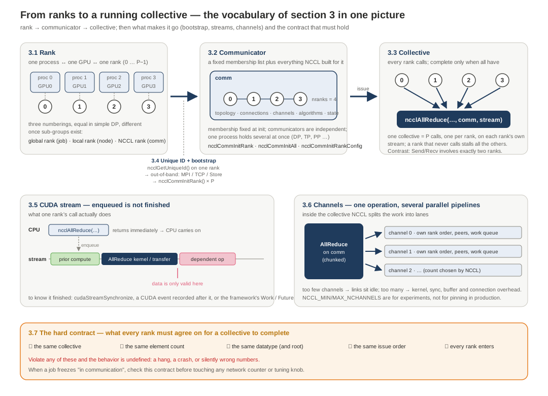
The whole section in one picture — read the top row left to right (ranks are grouped into a communicator, which issues collectives), then the mechanics underneath (how the communicator is bootstrapped, what a call does on a CUDA stream, how the work splits into channels), and finally the contract every rank must honor:
3.1 Rank
A rank is a participant’s number inside one communication group, 0 … nranks−1. The common mapping is one process ↔ one GPU ↔ one NCCL rank — not an NCCL requirement (one process can drive several GPUs with one communicator each), but the easiest to manage for CUDA contexts, CPU affinity, and fault isolation. Three numberings must not be confused:
- Global rank — the process number across the whole job.
- Local rank — the number within one node, usually used to pick the local GPU.
- NCCL rank — the number inside one particular communicator.
They coincide in a simple data-parallel job, and diverge as soon as sub-groups exist: the tensor-parallel group and the data-parallel group each create their own communicator, and the same process can hold a different NCCL rank in each.
3.2 Communicator
The communicator is NCCL’s central object: a fixed set of ranks plus their topology, connections, channels, algorithms, and runtime state — a “communication room” with a membership list. Membership is fixed at initialization; every rank must enter the group’s collectives in a consistent order; different communicators are independent; one process typically holds several (DP, TP, PP…). Initialization comes in three flavors: ncclCommInitRank (multi-process/multi-node, the common case), ncclCommInitAll (single process driving several GPUs), and ncclCommInitRankConfig (with extra configuration; capabilities evolve by version).
3.3 Collective
A collective is an operation that every rank in the communicator takes part in: each rank calls the same function — ncclAllReduce, ncclBroadcast, … — against the same communicator, and the operation is only complete when all of them have. AllReduce is everyone doing AllReduce together; nobody is optional, and no rank can be a passive bystander. That is the contrast with point-to-point Send/Recv, where exactly two ranks are involved and the rest of the group is unaware. Three consequences follow directly:
- Each rank issues the call on its own stream, so a collective is really one submission per rank that NCCL stitches into a single operation.
- A rank that never makes its call stalls every other rank forever — which is why “one rank hung” presents as “the whole job hung”.
- The order in which collectives are issued must agree across ranks: NCCL matches them by position in the issue sequence (the API has no tags or ids) — the rule made precise in 3.7.
3.4 Unique ID and bootstrap
One process calls ncclGetUniqueId(), then distributes the ncclUniqueId to all others through a control plane outside NCCL — MPI broadcast, TCP socket, the PyTorch Store, or the rendezvous mechanism of Kubernetes or the job launcher. Everyone then calls ncclCommInitRank() with the same ID, a consistent nranks, and its own rank. The ID is how members of the same group find each other; during bootstrap NCCL exchanges node, GPU, NIC, and connection information, then builds the actual transport channels. The division of labor matters for debugging: NCCL owns the data plane; member discovery, process launch, and ID distribution belong to the upper runtime.
After the ID exchange, bootstrap proceeds into connection establishment — the full sequence, from ID distribution to buffer allocation, is section 8.6, and the topology discovery that informs it is section 8.1.
3.5 CUDA streams: enqueued is not finished
NCCL calls take a CUDA stream, and when the call returns, the operation has usually only been enqueued — no data has necessarily moved:
CPU calls ncclAllReduce
        ↓
communication work is enqueued on the CUDA stream
        ↓
GPU waits for preceding computation to finish
        ↓
communication kernel executes / transfer is driven
        ↓
subsequent dependent operations may continue
To know a transfer finished: synchronize the stream, wait on a CUDA event recorded after it, or use the framework’s async Work/Future interface. A separate communication stream lets communication overlap independent computation — but the dependency must then be expressed explicitly with events or stream waits.
3.6 Channels
NCCL splits one operation across multiple channels — logical communication pipelines, each with its own rank ordering, peer connections, and work queues; lanes on a highway. Too few channels underutilize NVLink or NIC bandwidth; too many inflate kernel, synchronization, buffer, and connection overhead. NCCL picks the count automatically; NCCL_MIN/MAX_NCHANNELS exist for diagnostics and experiments, not for blind pinning in production.
3.7 The hard contract
One rule explains most training hangs: within a single collective, every rank must pass the same element count and datatype, enter the same operation, in the same order — and every rank must actually enter the call. Violate it and behavior is undefined: hang, crash, or silently wrong numbers. When a job freezes “in communication”, the first check is not a network counter; it is whether some rank skipped the call, reordered two collectives, or passed a mismatched shape.
Notation below: P = ranks in the communicator, N = elements per shard, S = bytes per element.
4. The primitives
NCCL’s native interface has long covered five collectives — AllReduce, AllGather, ReduceScatter, Broadcast, Reduce — plus point-to-point Send/Recv; NCCL 2.28 (September 2025) added native host APIs for the remaining three patterns, ncclAlltoAll, ncclGather, and ncclScatter. On older releases those patterns are composed from grouped point-to-point operations, and whether a same-named framework API maps to the native function or a grouped-P2P composition still depends on the framework and version — treat the documentation of the version you run as authoritative. Conceptually the whole zoo sorts into three families by two questions: does the data get reduced, and who ends up holding the result?
4.1 Reduction family: AllReduce, Reduce, ReduceScatter
Reduction means combining corresponding elements from all ranks with one operator — sum, prod, min, max, avg. The three members differ only in who keeps the result, and whether it is sliced:
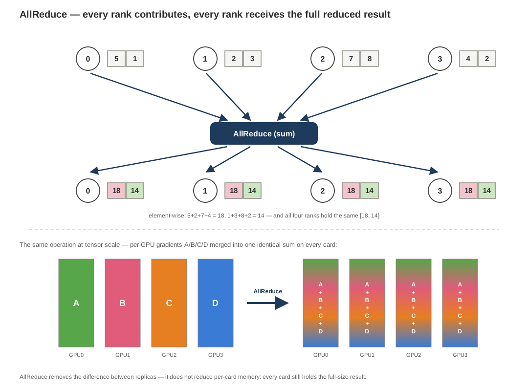
- AllReduce — every rank contributes an equal-size tensor; afterwards every rank holds the complete reduced result. The workhorse of data parallelism: PyTorch DDP AllReduces gradient buckets during the backward pass so every replica applies identical updates; tensor parallelism uses it to merge partial matrix products. One property worth stating precisely: AllReduce eliminates the difference between model replicas, but saves no memory — every card still holds full parameters, full gradients, and usually full optimizer state. It solves synchronization, not sharding.
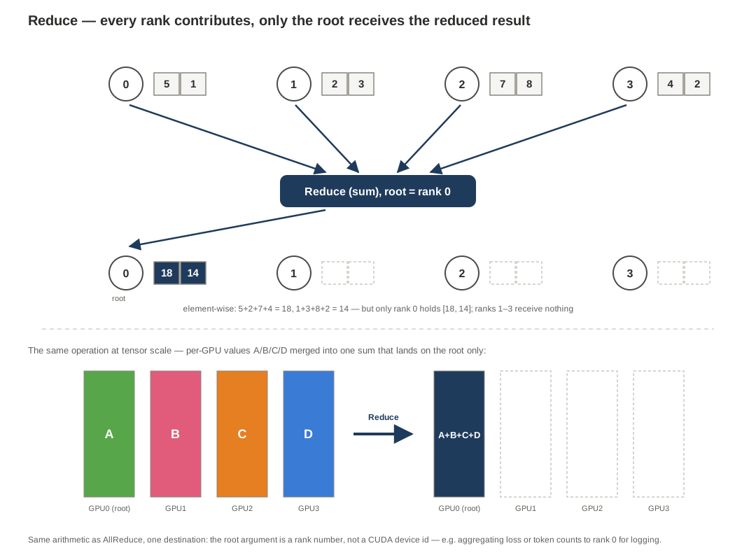
- Reduce — same arithmetic, but only the root rank keeps the result (the root argument is a rank number, not a CUDA device id). For “one place needs the answer”: aggregating loss or token counts to rank 0 for logging.
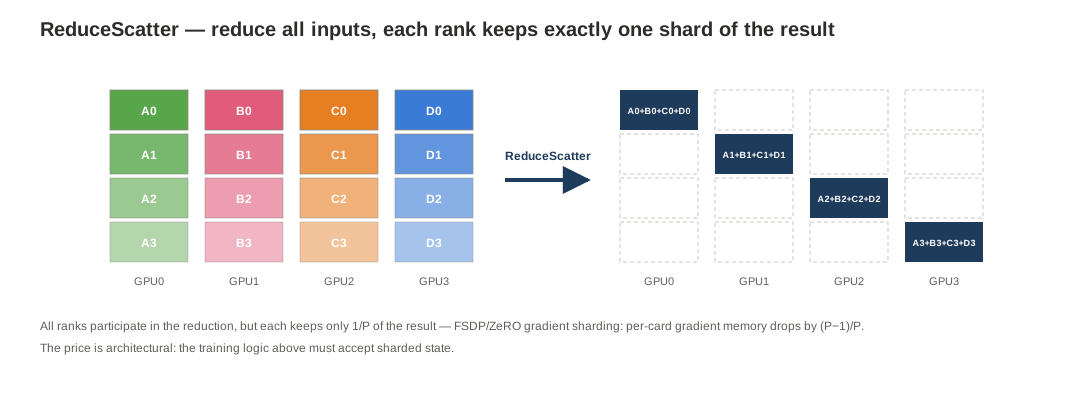
- ReduceScatter — reduce everything, then slice the result into P blocks; rank i keeps block i. The natural primitive for sharded training (FSDP/ZeRO): if a rank only owns 1/P of the parameters, it only needs 1/P of the reduced gradients — gradient memory drops by (P−1)/P. The price is architectural: the training logic above must accept that state lives sharded.
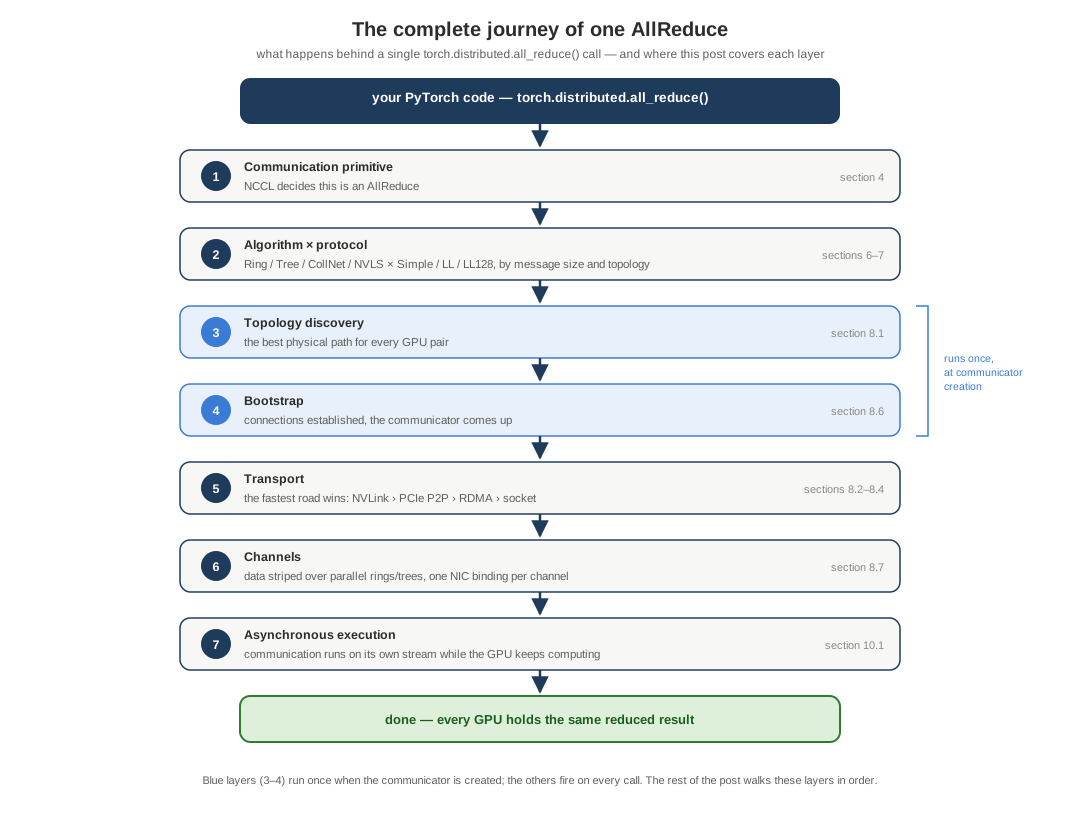
Since AllReduce is the workhorse, it also makes the best preview of everything this post covers — the complete journey behind one torch.distributed.all_reduce() call, with the section that covers each layer:
4.2 Collect-and-distribute family: Broadcast, Scatter, Gather, AllGather
This family does no arithmetic — it only moves data. The four members are distinguished by one question: where does the complete data start, and where does it end up?
- Broadcast — the root has the full tensor; afterwards everyone has a copy. Used at startup: rank 0 loads or initializes weights, broadcasts them, and every replica starts from identical state; also configuration and checkpoint distribution.
- Scatter — the root holds P chunks and hands chunk i to rank i — distribution with slicing.
- Gather — the reverse: every rank’s chunk is collected to the root only — for example, pulling scattered eval results onto one card.
- AllGather — every rank contributes its shard, and every rank receives the full concatenation, ordered by rank index. FSDP’s other half: parameters live sharded; just before a layer computes, an AllGather temporarily reassembles the full weights, which are released after use. The cost is just as characteristic: the full tensor materializes on every rank, so AllGather timing is exactly the knob FSDP tunes to keep peak VRAM under control.
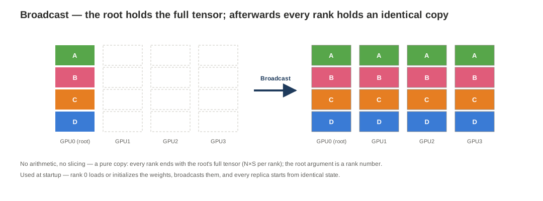
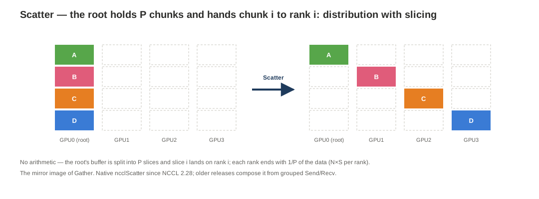
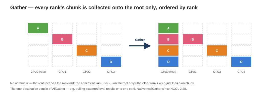
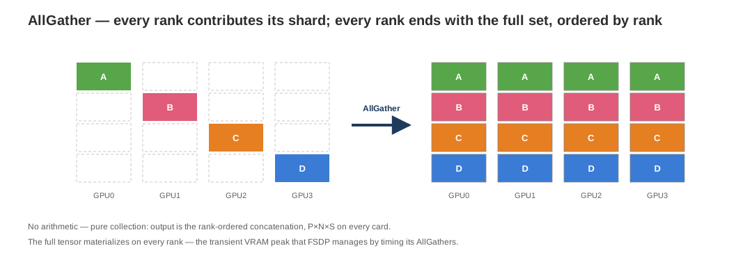
A one-line mnemonic for the whole zoo: “All-” means every rank ends with the final result; “Reduce” means arithmetic happened; “Scatter” means the result was sliced and distributed. Communication volume in this family is on the order of (P−1) × N × S per rank.
AllReduce vs AllGather, side by side
The shared “All-” prefix is exactly why these two are the most-confused pair in the zoo: both end with every rank holding identical content, so the picture “afterwards, everyone has everything” fits either. They differ on every other axis:
| AllReduce (4.1) | AllGather | |
|---|---|---|
| Each rank contributes | a full-size tensor — P same-shaped versions of the same quantity (P gradients) | one shard — the i-th 1/P piece of a tensor no rank holds in full |
| Arithmetic | yes — element-wise: out[i] combines every rank’s in[i] (sum, max, …) | none — bytes are copied, never combined |
| Element i of the result | depends on all P ranks’ values at position i (their sum — or the max among them) | comes from exactly one rank — the one whose shard covers position i |
| Result size per rank | equal to each input — nothing grows | P×N×S — grows P-fold, concatenated in rank order |
| Typical job | merge DDP’s gradient replicas | reassemble FSDP’s sharded parameters |
The instinct to keep: AllReduce answers “we each computed a version of the same thing — combine them”; AllGather answers “we each hold a different piece — hand everyone the whole.” The figures above carry the same distinction in color: AllGather’s output keeps every shard’s color, because the data only moved; AllReduce’s output turns a single dark color, because the inputs were merged and the originals are gone. It is also why the identity in section 6.1 decomposes cleanly — ReduceScatter performs all of the arithmetic and leaves the result sharded; the AllGather half only moves finished pieces and never touches a value.
4.3 Full-exchange: AlltoAll
AlltoAll is the only true everyone-to-everyone exchange: rank i sends its j-th chunk to rank j and receives one chunk from every peer. Treat the P send buffers as a P×P block matrix and AlltoAll is a distributed transpose. Its main stage is Mixture-of-Experts: tokens are routed to whichever rank hosts their expert (dispatch), computed, then routed back (combine) — two AlltoAlls per MoE layer in forward, two more in backward. Its traffic is scattered by nature and highly sensitive to bisection bandwidth, congestion control, and load balancing. Three sharp edges: it is data rearrangement, not reduction; real token routing is naturally uneven and there is no AlltoAllV-style variable-count collective, so MoE frameworks often build variable-length exchanges from grouped send/recv rather than a fixed-size AlltoAll; and the fixed pattern does not run in place — send and receive buffers must be separate, peak user memory 2 × P × N × S.
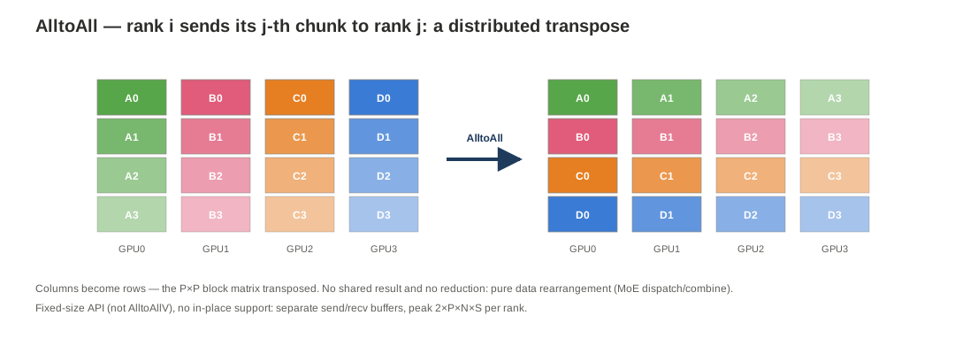
4.4 send/recv: when the pattern is not collective at all
Pipeline parallelism’s traffic — stage k handing activations to stage k+1, gradients flowing back — is point-to-point, and NCCL provides plain send/receive for it: adjacent-stage activation passing, irregular exchanges, AlltoAll composition, directed tensor transfers in inference systems. Any irregular pattern can be built from it, at a cost: who sends, who receives, in what order, with what buffers, and how communication overlaps compute all become your design problem. One mechanical rule from the API: mutually dependent Send/Recv operations must be submitted as one group between ncclGroupStart() / ncclGroupEnd() — it avoids serialized-submission deadlocks and lets NCCL plan the whole set at once.
5. From primitive to parallelism
5.1 Which parallelism calls which primitive
| Parallelism / framework | Main communication | When it fires | Message profile |
|---|---|---|---|
| DDP (data parallel) | AllReduce | During backward, per gradient bucket | Large messages, fewer calls — bandwidth-bound |
| FSDP / ZeRO | AllGather + ReduceScatter (some scenarios AllReduce) | Per layer, forward and backward | Medium messages, many calls — overlap-dependent |
| Tensor parallel (TP) | AllReduce / AllGather / RS | Every layer, forward and backward | Very frequent, latency-critical |
| Pipeline parallel (PP) | send/recv | Between adjacent stages | Point-to-point, overlaps with compute |
| MoE (expert parallel) | AlltoAll / grouped send-recv | 2× forward + 2× backward per layer | Many small uneven messages — latency/balance-bound |
| Sequence parallel | AllGather + ReduceScatter | Around attention/norm boundaries | Follows TP’s frequency profile |
The diagnostic value: when communication is the bottleneck, first find your row. DDP wants big-message bandwidth; MoE wants small-message latency and even load distribution. Those are optimized in opposite directions, and tuning for the wrong row is wasted work. It is also why benchmarking only AllReduce cannot represent training performance — MoE systems in particular need AlltoAll measured under imbalanced token distributions.
5.2 Memory: three layers before quoting any number
“How much memory does a collective use?” has no single answer — it has three layers:
- User buffers — determined by semantics, exactly computable. AllGather’s output is inherently
P×N×Son every rank; fixed AlltoAll peaks at2×P×N×S. The savings lever is in-place operation, and NCCL specifies the conditions exactly: AllReduce/Reduce/Broadcast are in-place whensendbuff == recvbuff; AllGather when the send buffer sits atrecvbuff + rank × sendcount; ReduceScatter when the receive buffer sits atsendbuff + rank × recvcount; AlltoAll never. - NCCL’s internal buffers — transit buffers per connection (
NCCL_BUFFSIZE, default 4 MiB), but the true total scales with channel count, connections, protocol, and topology, and every extra communicator (process group) adds a full set. The only accurate accounting is differential: readcudaMemGetInfobefore/after communicator init and before/after the first collective. - Framework accounting — PyTorch’s
memory_allocatedtracks only its own caching allocator; NCCL allocates outside it and is invisible there. Mixing the two ledgers produces confident wrong conclusions.
Practical summary: the dominant term is almost always layer 1 — AllGather’s P×N×S grows with model size and communicator width, which is why FSDP limiting how many layers are gathered simultaneously saves more memory than any NCCL knob.
5.3 Don’t memorize APIs — follow the tensor’s fate
The most useful judgment framework: pick (or recognize) a primitive by asking is this tensor replicated, sharded, or being redistributed?
- Every GPU has a gradient, every GPU needs the same merged result → AllReduce
- Every GPU needs only its own slice of the merged result → ReduceScatter
- Every GPU holds a slice, the next computation needs the whole tensor → AllGather
- One root hands the same data to everyone → Broadcast (sliced per rank: Scatter)
- Everyone’s data converges on one root → Reduce (without arithmetic: Gather)
- Every rank exchanges a different slice with every other rank → AlltoAll
- The pattern is irregular, or strictly stage-to-stage → send/recv
6. Algorithms: how a collective is organized across ranks
6.1 The one equivalence worth memorizing
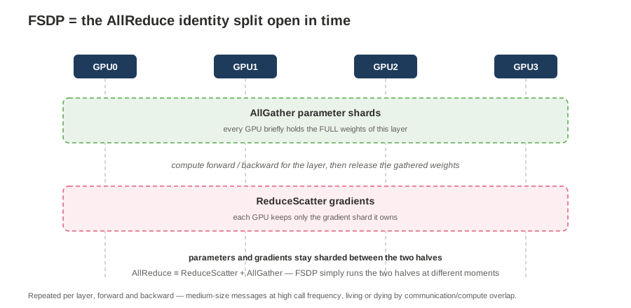
AllReduce ≡ ReduceScatter + AllGather
First everyone reduces and keeps one slice; then everyone gathers all slices back. High-performance Ring AllReduce is implemented exactly along these lines — not “reduce centrally, then broadcast”. FSDP is this same identity deliberately split open, running the two halves at different times so parameters and gradients stay sharded in between:
6.2 Ring
The Ring algorithm arranges P ranks in a logical ring and cuts a message of M bytes into P chunks:
Rank 0 → Rank 1 → Rank 2 → Rank 3
  ↑                          ↓
  └──────────────────────────┘
- Phase 1 — ReduceScatter: each rank sends a chunk to its neighbor; each received chunk is reduced with the local data and passed on. After P−1 steps, every rank holds one chunk of the final result.
- Phase 2 — AllGather: each rank forwards its finished chunk around the ring; after another P−1 steps everyone has everything.
Step through it on four GPUs. Assume each GPU starts with four chunks of its own data:
GPU0 has [a₀, b₀, c₀, d₀]
GPU1 has [a₁, b₁, c₁, d₁]
GPU2 has [a₂, b₂, c₂, d₂]
GPU3 has [a₃, b₃, c₃, d₃]
⊕ is the reduction, and the goal is for every GPU to end with [A, B, C, D], where A = a₀⊕a₁⊕a₂⊕a₃ and likewise for B, C, D. Watch the ring do it in three reduce-scatter hops followed by three all-gather hops — six steps in all — the two P−1 phases above, 2(P−1) together:
Per-rank transfer volume is 2 × (P−1)/P × M — approaching 2M as P grows. For the 8-GPU, 14 GB-gradient example from section 1: ~24.5 GB through the links per rank per step, more than the gradient tensor itself, repeated every step. That is the “communication wall” of large-scale training. Ring’s strengths: no central bottleneck, every link busy, fully pipelined — ideal for large bandwidth-dominated messages on a modest number of nodes. Its weakness: about 2(P−1) communication steps, so for small messages the accumulated latency dominates as P grows.
6.3 Tree
Tree AllReduce reduces up and broadcasts down a tree, so its step count grows with the tree’s height rather than with the rank count — better for small, latency-sensitive messages, and for large scale. What NCCL actually builds (since 2.4) is a double binary tree across nodes, with a chain through the GPUs inside each node (one chain per NIC). The tree’s vertices are nodes, not GPUs, and the two trees are complementary: every node is an interior vertex in at most one of them (one node may be a leaf in both), and each tree carries half the data. That is what restores full bandwidth — a single binary tree would leave its leaves sending only during the reduce and receiving only during the broadcast, wasting half of every link. Chunking, pipelining, and multiple channels keep every link busy, and the two trees have different roots, so no node is a hotspot. “Tree” does not mean all data funnels through one fixed root — and in NCCL it is AllReduce-only. (How it compares to Ring in measured numbers is in 6.6.)
Same four GPUs and the same starting data as the Ring walkthrough above, now arranged as a tree: GPU0 is the root, GPU1 and GPU2 are its children, and GPU3 hangs below GPU2. Round 1: GPU1→GPU0 and GPU3→GPU2 run in parallel, producing the subtree partials V₀₁ and V₂₃. Round 2: GPU2 sends V₂₃ up and the root computes V₀₁ ⊕ V₂₃ = [A, B, C, D]. Then the result is broadcast back down in two more rounds. Four steps instead of Ring’s six — the logarithmic advantage. Two things this teaching tree simplifies: every hop carries a whole vector, where Ring’s hops carry 1/P-sized chunks — which is exactly why real NCCL chunks and pipelines its trees; and it is a single tree drawn over GPUs, where NCCL runs two complementary trees between nodes with a chain inside each node:
6.4 CollNet
CollNet is the family of algorithm paths that use network-side collective offload — switches or fabric services that can aggregate during transmission — combining intra-node reduction, in-network aggregation, and intra-node distribution to cut the cost of cross-node collectives. Whether it is available depends on NCCL version, network hardware and drivers, the NCCL Net/CollNet plugin, the SHARP Aggregation Manager (under UFM) or equivalent vendor components, and the current topology and scale. Setting NCCL_COLLNET_ENABLE=1 is necessary but not sufficient: without the plugin, a SHARP-capable fabric, and at least two nodes, NCCL silently falls back to Ring and Tree.
GPU reductions inside each node
              ↓
collective reduction across nodes
              ↓
distribution back to every local GPU
The key distinction is that CollNet hands the inter-node phase to a collective-network plugin. The plugin exposes operations such as an asynchronous iallreduce(). With NVIDIA SHARP, that collective is reduced inside the network switches; another CollNet plugin could implement it differently. CollNet itself is therefore an NCCL interface and algorithm family — not necessarily switch hardware.
The four-GPU walkthrough: CollNetDirect
The same four GPUs and starting data once more, now split across two nodes — Node A holds GPU0/GPU1, Node B holds GPU2/GPU3 — joined by two CollNet reduction rails (a rail is one head-GPU-to-HCA path into the fabric; defined fully below). Inside each node one GPU acts as the head for each rail:
Node A                          Node B
GPU0 = head 0                   GPU2 = head 0
GPU1 = head 1                   GPU3 = head 1

head / rail 0 owns a,b
head / rail 1 owns c,d
Each GPU first scatters its non-owned slice to the matching local head; each head reduces its two local contributions and uploads a single node-level partial on its rail; the fabric reduces the two node partials in the network and hands [A, B] or [C, D] back to the heads; finally the heads exchange slices locally so every GPU assembles [A, B, C, D]. Four steps, and only one partial per node per rail ever crosses the inter-node link — that is the bandwidth saving the offload buys.
Note: this is a demo assignment — see “What the visualization intentionally simplifies” below for what real NCCL does with chunks, heads, and channels.
What a “head” actually means
A head is a GPU rank selected by NCCL as the endpoint for a collective-capable NIC or network rail. It is not necessarily GPU0, and it is not a global root. For CollNetDirect:
- NCCL discovers one or more heads in each node.
- Every local GPU connects to the available heads.
- Each head connects back to all its local peers.
- Tensor chunks are striped across the heads.
- NCCL rotates assignments so all GPUs do not target the same head simultaneously.
In the source these concepts are represented by nHeads, headRank, up, down, and shift (struct ncclDirect in src/include/device.h).
A rail is the logical path formed by corresponding heads and HCAs across nodes (HCA — Host Channel Adapter — is the RDMA-capable network adapter used for InfiniBand or RoCE between machines). Multi-rail SHARP deployments generally need equivalent HCA rails on every server so that they connect through corresponding parts of the fabric.
CollNetDirect versus CollNetChain
| Property | CollNetDirect | CollNetChain |
|---|---|---|
| Local topology | Multi-head fan-in / fan-out | Linear GPU chain |
| Chunk ownership | Striped across several heads | One head per channel |
| Local path depth | Shallow | Grows with GPUs per node |
| NIC parallelism | Can use multiple rails concurrently | Channels may use different heads |
| Main cost | Requires rich local connectivity | Serial local forwarding |
| Natural fit | Dense NVLink/NVSwitch and balanced NIC topology | Less densely connected topology |
CollNetChain reduces along a local chain, sends the node result through the collective network, then broadcasts back down the chain. CollNetDirect uses multiple heads to eliminate that long local chain. NCCL enables CollNetDirect only on NVSwitch systems, where the any-to-any intra-node bandwidth it relies on exists; CollNetChain is the option everywhere else. (CollNet arrived in NCCL 2.6; the Chain/Direct split in 2.14.)
What the visualization intentionally simplifies
The five displayed states are dependency stages for one set of chunks. A real NCCL operation does not globally finish every scatter before starting the network phase. NCCL:
- splits the tensor across multiple channels;
- further divides channels into chunks;
- stripes chunks across multiple heads;
- assigns separate CUDA thread groups to scatter, reduce, broadcast, and gather;
- uses an asynchronous proxy to issue the network collectives.
Consequently, while chunk k is being reduced by the network, chunk k+1 may be undergoing local reduction and chunk k+2 may already be scattering. This pipeline is essential for bandwidth.
When CollNet performs well
CollNetDirect is most attractive when:
- the job spans multiple nodes (CollNet is never used on one node —
NCCL_COLLNET_NODE_THRESHOLDdefaults to 2); - a collective-network plugin such as the NVIDIA SHARP plugin (
nccl-rdma-sharp-plugins) is installed, andNCCL_COLLNET_ENABLE=1is set — CollNet is off by default; - GPUDirect RDMA works correctly;
- local GPU-to-GPU links are fast;
- GPUs have well-balanced access to NICs;
- matching HCA rails exist across the nodes;
- messages are large enough to amortize setup and the local scatter/gather.
The current NCCL cost model specifically notes that CollNetDirect needs every GPU to have a local NIC path to run at full speed; fewer heads can still support an all-reduce, but they concentrate the work on those heads.
6.5 NVLS
On platforms with NVLink SHARP (NVLS) capability, part of the reduction executes inside the NVSwitch fabric itself, reducing the data shuttled redundantly between GPUs — for collectives within a node, and specific multi-node cases. Like CollNet it depends on the GPU generation, NVSwitch platform, driver, Fabric Manager, and NCCL version; a PCIe GPU server cannot obtain NVLS through software configuration.
NVLS is an in-fabric reduction mechanism inside NVSwitch: a GPU initiates the operation, but NVSwitch hardware performs the cross-GPU reduction and multicast. That is the key difference from CollNetDirect:
CollNetDirect : local GPU heads perform the node reduction
NVLS          : NVSwitch performs the node reduction
NVLS requires a multicast-capable NVSwitch system — third-generation NVSwitch / NVLink 4 with Hopper or later — not merely a Hopper PCIe GPU. It arrived in NCCL 2.17 as an intra-node AllReduce (today it also serves AllGather and ReduceScatter); 2.18 added the multi-node forms — NVLS inside the node chained with IB SHARP between nodes (plain NVLS), and NVLSTree (NVLS inside the node, NCCL’s double binary tree between nodes, AllReduce-only), which needs no IB SHARP at all. What it buys, in numbers, is in 6.6.
The two hardware operations
NVLS relies on CUDA multicast memory and two PTX operations:
| Operation | Meaning |
|---|---|
multimem.ld_reduce | Read the same address from every GPU replica, reduce those values in NVSwitch, and return one result |
multimem.st | Write one value to the same address on every GPU replica — a hardware multicast |
A multicast address does not refer to one physically shared buffer. It refers to a multicast object backed by one physical memory replica on each participating GPU:
         one multicast virtual address
                      │
        ┌──────┬──────┼──────┬──────┐
        ▼      ▼      ▼      ▼      ▼
      GPU0   GPU1   GPU2   GPU3   …
    replica replica replica replica
CUDA creates the multicast group, adds the participating GPUs, binds each GPU’s physical memory to it, and exposes a multicast virtual address (cuMulticastCreate → cuMulticastAddDevice → cuMulticastBindMem → mapped into each GPU’s address space).
The four-GPU walkthrough: NVLS
The same four GPUs and starting data one last time, now hanging off a single NVSwitch. Every GPU keeps a local UC (unicast) backing replica of the buffer, and one MC (multicast) address is mapped over all four replicas at matching offsets. For the teaching slice, GPU0 owns stripe a, GPU1 owns b, GPU2 owns c, GPU3 owns d. The four steps:
- Each GPU stages its four stripes into its own UC replica.
- Each owner issues a
multimem.ld_reduceat the MC address for its stripe — the switch reads that stripe from all four backing replicas, reduces them in the fabric, and returns one result to the issuing GPU. - Each owner issues a
multimem.stat the MC address — the switch writes the finished stripe into a second, receive-side UC replica on all four GPUs at once. - Every GPU reads
[A, B, C, D]from its own local replica.
No GPU ever sends a chunk to another GPU — the reduction and the broadcast both happen inside the switch:
6.6 Don’t pin the algorithm
NCCL builds a performance model from message size, rank count, node count, topology, link bandwidth, and available plugins, then chooses per collective. The rough tendencies:
| Scenario | Direction that tends to win |
|---|---|
| Small messages, latency-sensitive | Tree (the cost model picks LL / LL128 at those sizes) |
| Large messages on few nodes, bandwidth-sensitive | Ring |
| Hundreds of GPUs and up, any size | Tree (or NVLSTree) — ring latency and bandwidth both degrade with scale |
| Network collective offload available | CollNet / the corresponding plugin path |
| NVLink SHARP available | NVLS |
These are rules of thumb, not rules — the heuristics change across versions. NCCL_ALGO is for A/B testing and fault isolation, not a standing optimization.
Ring vs Tree vs CollNet vs NVLS at a glance
The comparison below is rebuilt from primary sources — NVIDIA’s NCCL 2.4 post on double binary trees, the NCCL user guide, the NCCL source’s tuning model and release notes, and the Hopper/NVSwitch architecture posts — because the popular three-column version of this chart gets several things wrong (see the note at the end).
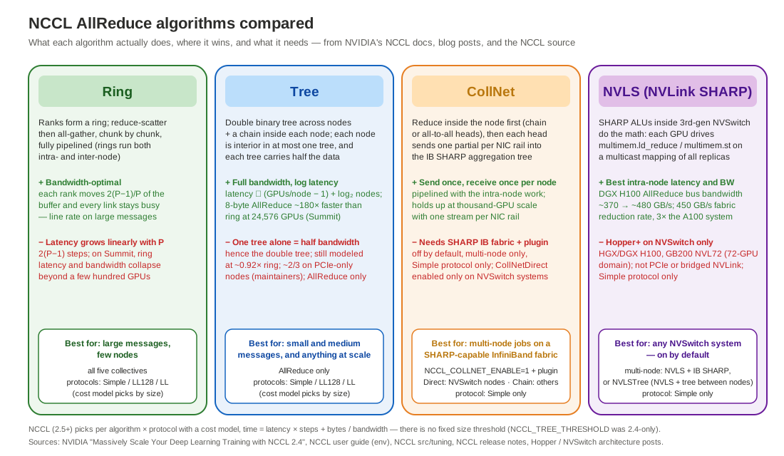
- Ring — Mechanism: ranks form a ring (NCCL’s rings run both inside and between nodes) and the data moves chunk by chunk through the two pipelined phases of 6.2, reduce-scatter then all-gather. Strength: bandwidth-optimal — each rank sends and receives only
2(P−1)/Pof the buffer and every link stays busy, so large messages run at line rate. Weakness:2(P−1)steps, so latency grows linearly with the rank count. In NVIDIA’s Summit measurements (NCCL 2.3 rings against 2.4 trees) an 8-byte ring AllReduce went from ~180 µs at 96 GPUs to ~45 ms at 24,576, and even 64 MB ring bandwidth collapsed from ~19 GB/s to under 2 GB/s over the same range. Applies to: all five collectives; all three protocols, chosen by size. Best for: large messages on a modest number of nodes. - Tree — Mechanism: as 6.3 explains, a double binary tree over nodes with a chain through each node’s GPUs; the two trees are complementary and each carries half the data. Strength: full bandwidth with logarithmic latency — latency ∝ (GPUs per node − 1) + log₂(nodes). On Summit the 8-byte AllReduce was ~180× faster than ring at 24,576 GPUs, and 64 MB bandwidth held at ~12–15 GB/s where rings had fallen below 2 GB/s. Weakness: the tuner models Tree at ~0.92× its ring-equivalent bandwidth, and on PCIe-only nodes NCCL’s maintainers put it at ~2/3, because the intra-node chain shares the PCIe link with the NIC — which is why tuning switches to rings earlier there. Applies to: AllReduce only; all three protocols. Best for: small and medium messages, and anything at scale.
- CollNet — Mechanism: the inter-node phase is handed to a network plugin (
ncclCollNet_t; the only publicly available implementation is NVIDIA’s SHARP plugin for Quantum InfiniBand switches). GPUs reduce inside the node first — a chain (CollNetChain) or an all-to-all across head GPUs (CollNetDirect) — then each head sends the node’s partial once per NIC rail into the switches’ SHARP aggregation tree, receives the result once, and redistributes it locally. It is not “every GPU to one switch in one hop”: only the heads talk to the network, and only after local reduction. Strength: each node sends its data once and receives the result once, pipelined with the intra-node work, so it holds up at thousand-GPU scale. Weakness: needs a SHARP-capable InfiniBand fabric plus the plugin, and NCCL only runs CollNetDirect on NVSwitch nodes (6.4). Applies to: AllReduce, AllGather, ReduceScatter (Direct); AllReduce (Chain); multi-node only; Simple only. Best for: multi-node training on a SHARP fabric. - NVLS (NVLink SHARP) — Mechanism: SHARP ALUs inside third-generation NVSwitch do the arithmetic. Each GPU owns a 1/P slice and drives
multimem.ld_reduce(the switch fetches that slice from every GPU’s replica and returns the sum) followed bymultimem.st(the switch multicasts the result back to every replica) — a reduce-scatter and all-gather performed by the switch, as the 6.5 walkthrough shows. Strength: the best intra-node latency and bandwidth: NCCL’s maintainers quote single-node AllReduce bus bandwidth on DGX H100 rising from ~370 to ~480 GB/s once NVLS is used (the normalized nccl-tests figure of 12.1, not wire throughput — the wire rate is the 450 GB/s of section 9.1), and NVIDIA rates the H100 NVSwitch fabric at 450 GB/s for reductions, 3× the A100 generation. Weakness: Hopper-or-later GPUs on an NVSwitch (NVLink 4+) system only — HGX/DGX H100 and GB200 NVL72, where the domain grows to 72 GPUs; PCIe cards and bridge-connected NVLink get nothing. Applies to: AllReduce, AllGather, ReduceScatter (NVLSTree: AllReduce only); Simple only. Multi-node: NVLS inside the node chained with IB SHARP between nodes (plainNVLS), or with NCCL’s double binary tree between nodes (NVLSTree, 2.18+), which needs no IB SHARP. On by default (NCCL_NVLS_ENABLE=2).
How NCCL actually chooses between them: since 2.5 there is no size threshold (NCCL_TREE_THRESHOLD lived only in 2.4). A cost model estimates time = latency × steps + bytes / bandwidth for every algorithm × protocol pair from per-topology tables and runs the cheapest — which is why a single job routinely uses Tree and Ring with all three protocols across its different message sizes. The tendencies that fall out of it: trees for small and medium sizes and at scale, rings for large sizes on few nodes (and on non-NVLink systems, trees only for small sizes), NVLS whenever the hardware allows.
What the popular three-column chart gets wrong (the one this figure replaces): its third column, labeled “CollNet”, describes NVLS — every GPU pushing to the NVSwitch chip, which does the sum — and claims it needs DGX-class NVSwitch hardware; CollNet proper is the InfiniBand SHARP path and needs no NVSwitch, while NVLS is the NVSwitch path. It states Tree runs at “half the bandwidth because only half the nodes work at each level” — true of one naive tree, not of NCCL’s double binary tree, which delivers full bandwidth. It draws Tree as a binary tree over GPUs, where NCCL’s tree is binary over nodes with a chain inside each node. It gives Ring “N−1 rounds” — that is one phase; AllReduce takes twice that, 2(P−1) in this post’s notation. And it pairs each algorithm with fixed protocols and fixed message sizes (“Ring + Simple/LL128 for ≥ tens of MB, Tree + LL/LL128 for ≤ a few MB”), where NCCL’s cost model picks the protocol per size for both algorithms — the one hard protocol rule is the Simple-only restriction on the offload algorithms, stated in section 7.
7. Protocols: Simple, LL, LL128
Algorithms describe how communication is organized between ranks; protocols describe the format, granularity, and synchronization of the data within each step.
- Simple — favors bandwidth: high payload ratio, efficient at link speed; the fixed overhead shows on small messages.
- LL (Low Latency) — every 8-byte store carries 4 bytes of data and a 4-byte flag, so the receiver sees readiness immediately and skips the synchronization waits; the flags cost half the bandwidth (LL tops out around 50% of peak), so NCCL uses it only for very small messages.
- LL128 — the compromise: a 128-byte line carries 120 bytes of data and an 8-byte flag, keeping fine-grained pipelining at ~95% of peak bandwidth. It relies on 128-byte stores being observed in order, so NCCL enables it only on paths where that holds — NVLink inside the node, and across the network when the NIC sits behind PCIe switches rather than a host bridge; Hopper and Blackwell extend that to the PXN and Grace C2C paths. Enabling it elsewhere can corrupt data, which is why the docs discourage touching
NCCL_PROTOat all.
Ring and Tree can each run all three protocols. The offload algorithms — CollNet, NVLS, and PAT (Parallel Aggregated Trees, the log-step AllGather/ReduceScatter algorithm added in 2.23) — are Simple-only.
The selection space is two-dimensional, and the full execution plan wider still:
algorithm : which ranks the data passes through, in how many steps
protocol  : how each step is packaged, synchronized, and pipelined

final execution plan = algorithm × protocol × channels × transport path
The same AllReduce may run Tree+LL in one size range and Ring+Simple in another. Like NCCL_ALGO, NCCL_PROTO is an isolation and experimentation knob, not a general optimization.
8. Topology: what NCCL discovers, and the paths it picks
8.1 Why topology matters, and what discovery does
Three numbers explain why NCCL’s first job is cartography:
| Path | Bandwidth | Analogy |
|---|---|---|
| NVLink 4.0 (H100) | 900 GB/s (aggregate, both directions) | high-speed rail |
| PCIe Gen5 x16 | ~64 GB/s per direction (~128 GB/s bidir) | national highway |
| NDR InfiniBand, per NIC | ~50 GB/s per direction (~100 GB/s bidir) | provincial road |
(Conventions labeled per section 9.1’s fact-check note.) Roughly an order of magnitude separates NVLink from everything else — if traffic that should ride NVLink ends up on PCIe, performance does not degrade, it collapses. So before anything moves, NCCL works out how every GPU is physically connected.
What a simplified two-socket server looks like from NCCL’s point of view:
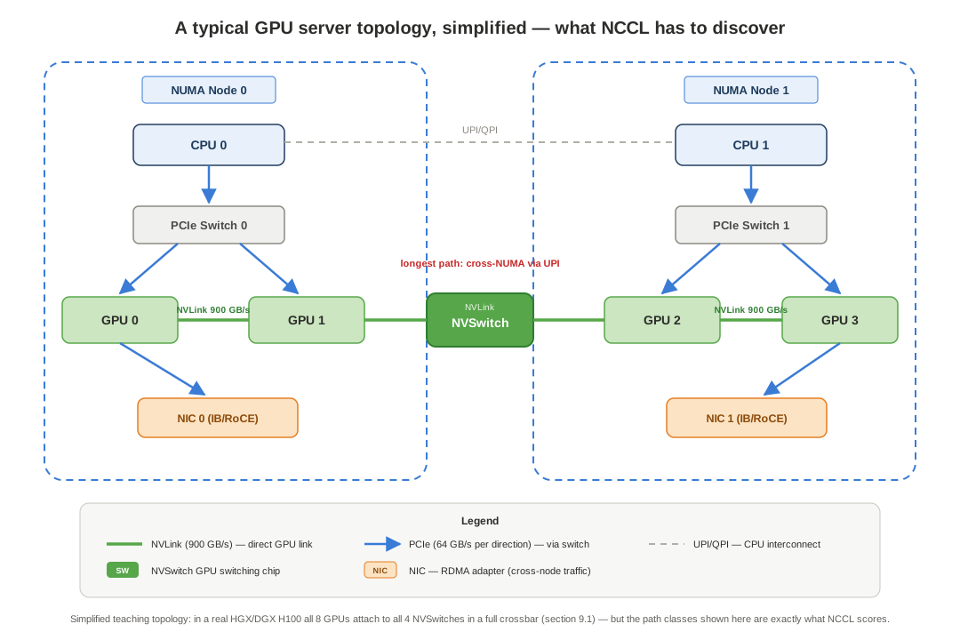
The key observations NCCL must extract from this map:
- GPU0 and GPU1 share NUMA node 0 and PCIe Switch 0, and also have a direct NVLink — two candidate paths roughly 7× apart in bandwidth (8.3).
- GPU2 and GPU3 mirror that under NUMA node 1.
- GPU1 and GPU2 are cross-NUMA, but the NVSwitch connects them at full NVLink speed — lower latency than PCIe despite crossing the socket boundary.
- GPU0 to GPU2/GPU3 over PCIe would be the worst path in the box: cross-NUMA and cross-PCIe-switch, through the CPUs’ UPI interconnect.
- Each NIC hangs off one PCIe switch — which is why GPU–NIC affinity (section 8.5) matters for cross-node traffic.
(The figure is a teaching simplification: in a real HGX/DGX H100 all 8 GPUs attach to all 4 NVSwitches in a full crossbar, as section 9.1 describes — but the path classes it shows are exactly what NCCL distinguishes.)
At communicator init, discovery runs in four steps:
- Enumerate the hardware — walk the PCIe tree via
/sys/devicesand the NVML API: GPU models, device numbers, CUDA capability; NVLink connections; the GPU–PCIe-switch–CPU–NUMA relationships; NICs/HCA ports and their PCIe distance to each GPU; P2P and GPUDirect RDMA capability; available network plugins. - Build the topology graph — which device sits under which switch, which NUMA node owns what.
- Score every GPU pair — the fastest path between each pair and its bandwidth class (the same classes
nvidia-smi topo -mprints: NVLink, same PCIe switch, across the host bridge, across NUMA). - Search communication graphs — build rings, trees, and NVLS structures over those scores, placing “near” GPUs adjacent in the ring order.
Like a courier who just moved to a new district: first study the map, then plan the routes. Every communicator that comes out of this process (section 3.2’s object, now filled in) holds:
- a topology-sorted rank list — the “nearest” GPUs placed adjacent in the communication order;
- the optimal ring/tree structures built over that list, one set per channel;
- a set of transport connections — for every pair that must talk, the fastest link available between them (NVLink, P2P, shared memory, RDMA, or socket).
With NCCL_DEBUG=INFO (plus NCCL_DEBUG_SUBSYS=INIT,GRAPH, section 13.1) the whole discovery is printed at startup — which NVLink pairs were found, which path class each connection got, which rings and trees were built over them. An excerpt from a real capture (two V100 nodes over InfiniBand, published in NVIDIA’s HPC-X manual; older NCCL, so the exact format varies by version):
# Using devices
#   Rank  0 Pid   7198 on  host1 device  0 [0x06] Tesla V100-SXM2-32GB
#   Rank  1 Pid   4890 on  host2 device  0 [0x06] Tesla V100-SXM2-32GB
host1:7198:7198 [0] NCCL INFO NET/IB : Using [0]mlx5_0:1/IB ; OOB ib0:1.1.21.3<0>
host2:4890:4920 [0] NCCL INFO GPU Direct RDMA Enabled for GPU 6000 / HCA 0 (distance 2 <= 3), read 0
host1:7198:7226 [0] NCCL INFO Ring 00 : 1[6000] -> 0[6000] [receive] via NET/UCX/0/GDRDMA
host1:7198:7226 [0] NCCL INFO Ring 00 : 0[6000] -> 1[6000] [send] via NET/UCX/0/GDRDMA
Three answers in four lines: which NIC was chosen (mlx5_0:1), whether GPUDirect RDMA engaged (and the topology distance that allowed it), and how the rings were built and over what transport (NET/UCX/0/GDRDMA). Reading this log against nvidia-smi topo -m is the fastest way to catch a wrong topology before it becomes a performance mystery (section 15.7). The operating-system view of the same facts:
nvidia-smi topo -m     ! GPU/NIC connectivity matrix: NVLink, same PCIe switch,
                       ! across host bridge, across NUMA - exact legend per driver version
8.2 One interface, many roads: the transport ladder
Discovery told NCCL what the map looks like; now the data has to actually travel. NCCL puts a unified transport interface over every physical link type, so an AllReduce that has passed through the algorithm layer never cares what it runs on — the transport layer picks the fastest implementation per GPU pair from the topology:
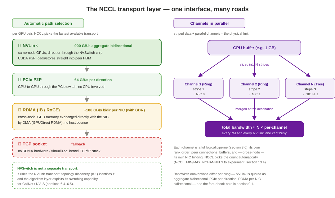
The selection logic, per pair, is a simple ladder: do the two GPUs share NVLink → use NVLink; else do they support PCIe P2P → use PCIe; else is there a configured RDMA NIC → use RDMA; else fall back to TCP sockets. All of it is automatic — no user intervention — and NCCL_DEBUG=INFO prints which transport each connection actually got (section 13.1). One subtlety the figure calls out: NVSwitch is not a separate transport. It rides the NVLink transport; topology discovery identifies it, and it is the algorithm layer that exploits its switching capability (CollNet/NVLS, sections 6.4–6.5).
8.3 Inside the node: NVLink, then PCIe P2P
When two GPUs in the same machine share NVLink, NCCL prefers it unconditionally. On an H100, NVLink 4.0 provides ~450 GB/s per direction (900 GB/s aggregate) — roughly 7× PCIe Gen5 x16 at matched conventions (the popular “14×” compares NVLink’s bidirectional total against PCIe’s one direction — the same convention mistake as 9.1’s fact-check note). NCCL uses CUDA’s P2P mechanism to read and write the peer GPU’s memory directly — no CPU, no system memory on the path. Analogy: an enclosed skybridge between two adjacent buildings — near, fast, and nobody goes outside.
Without NVLink (different-generation GPUs, or cards that only meet at a PCIe switch), NCCL falls back to PCIe P2P — the same CUDA P2P mechanism, running over the PCIe bus at ~64 GB/s per direction. Analogy: the street between the buildings — it gets you there, slower than the skybridge. When direct P2P is impossible (IOMMU, virtualization, container permissions), a shared-host-memory path steps in as the intermediary.
Two cautions from the earlier sections still apply: NVLink does not automatically translate into application performance — wrong rank-to-GPU binding, processes running across NUMA nodes, or a communication pattern that fights the topology still lose badly on top of perfect links.
8.4 Across nodes: RDMA, GPUDirect, and the proxy thread
When the GPUs sit in different machines, the data must cross the network, and NCCL uses RDMA — InfiniBand verbs or RoCE, or an NCCL Net plugin. The key property is GPUDirect RDMA (GDR):
without GPUDirect RDMA : GPU → CPU memory → NIC → network
with GPUDirect RDMA    : GPU ⇔ NIC → network
GPU memory → NIC → network → remote NIC → remote GPU memory, with the CPU and system memory never on the data path. That buys three things at once: lower latency (no CPU relay), higher bandwidth (no contention for CPU memory bandwidth), and lower CPU load (the CPU initiates, it does not move bytes). Analogy: RDMA is the direct flight between two cities, and GDR is the airport at your doorstep — no bus ride (CPU relay) to get there. “Direct” still does not mean bypassing PCIe: the PCIe/NUMA distance between GPU and NIC decides real performance, which is NCCL_NET_GDR_LEVEL’s whole job (section 13.2).
The part nobody sees on the GPU side is the proxy thread. For cross-node RDMA, NCCL runs a CPU-side proxy thread per GPU that listens for GPU-initiated transfer requests, manages RDMA connection setup and queue pairs (QPs), and handles network events — completion notifications and errors. The GPU never drives the NIC itself:
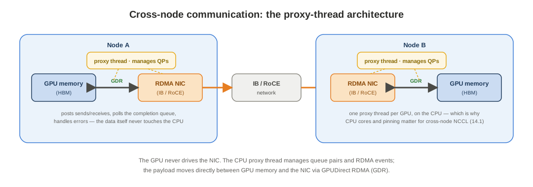
This is why CPU cores matter for cross-node NCCL (section 10’s phase 3, and 14.1): each GPU effectively needs a dedicated proxy thread, and a starved proxy stalls the NIC no matter how fast the fabric is.
And when none of the above exists — a virtualized environment, no RDMA-capable NIC — NCCL falls back to plain TCP sockets: the slowest road, and the most compatible one.
8.5 Multiple NICs and rails
High-end GPU servers carry multiple HCAs/NICs; NCCL assigns network paths by GPU–NIC topological distance and drives ports in parallel. The ideal mapping:
GPU 0/1 → nearby NIC 0
GPU 2/3 → nearby NIC 1
GPU 4/5 → nearby NIC 2
GPU 6/7 → nearby NIC 3
If a container exposes only some devices, NIC name selection is wrong, or CPU/GPU/NIC NUMA binding is off, traffic detours across sockets — link bandwidth drops and tail latency grows. This per-GPU-NIC layout is also exactly what the rail-optimized fabric design in section 9 exists to serve — and multi-rail only pays off when there are multiple channels to feed the NICs in parallel (section 8.7).
8.6 How connections are established (bootstrap)
Topology discovery tells NCCL what could connect; the GPUs still need actual connections before anything moves. That process is bootstrap:
- Generate the Unique ID — rank 0 calls
ncclGetUniqueId()and the ID is passed to every other rank through an external mechanism (MPI, environment variables, a shared file, the framework’s store — section 3.4). - Create the communicator — every rank calls
ncclCommInitRank()with the Unique ID and its own rank number. - Establish point-to-point connections — each GPU pair sets up a transport channel chosen from the discovered topology (NVLink/P2P, shared memory, RDMA, or socket), exchanging memory handles and port information.
- Allocate communication buffers — GPU memory buffers are allocated per channel for sends and receives.
In PyTorch all of this usually completes automatically behind torch.distributed.init_process_group() — with the wrinkle that the NCCL communicator is created lazily, at the first collective, so an “initialization” problem often surfaces at the first all_reduce instead. No engineer drives bootstrap by hand, but understanding it is what makes initialization-phase hangs and timeouts (section 15.1) debuggable. This is the front half of section 10’s initialization phase, seen from the connection side.
8.7 More than one road at once: channels stripe the data
Everything above is “how do two GPUs talk”. But a collective does not run on one ring: NCCL builds several parallel rings (or trees), each called a channel (section 3.6). The core idea is simple — if one ring cannot saturate the NVLink between GPU0 and GPU1, build two rings, cut the data in half, and run both at once. Concretely:
- NCCL stripes the buffer across the channels;
- each channel runs its own ring/tree with its own peers and buffers;
- all channels execute in parallel, and the summed bandwidth approaches the total of every available link (the right panel of 8.2’s figure).
Why channels earn their keep:
- load balance — a single ring touches only some links; more channels light up more parallel paths;
- multiple NICs — with two IB NICs per node NCCL typically builds at least two channels, each bound to its own NIC, which is what makes 8.5’s multi-rail real;
- NVSwitch topologies — many channels are how the all-to-all bandwidth of the crossbar actually gets utilized.
The channel count is chosen automatically from the topology; NCCL_MIN_NCHANNELS / NCCL_MAX_NCHANNELS exist for experiments (section 13.4 — their pre-2.5 names were NCCL_MIN_NRINGS/NCCL_MAX_NRINGS).
Which leaves the last question of the pipeline: what is the GPU doing while all this communication runs — waiting, or computing? That is the stream-and-overlap story of section 10.1.
9. NVLink and NVSwitch: the two domains of an AI cluster
9.1 The Scale-Up domain: NVLink and NVSwitch
NVLink is NVIDIA’s dedicated GPU-to-GPU interconnect, and architecturally it is not “a faster Ethernet” — it is a separate system that bypasses every layer a network engineer normally instruments: not the PCIe bus, not the RDMA NIC (ConnectX-6/7), not the OS network stack, not any switch you manage. Data moves from one GPU’s HBM directly into another GPU’s HBM; the CPU, the NICs, and your fabric are not on the path.
Inside an H100 SXM server the 8 GPUs are not pairwise-cabled: they interconnect through 4 NVSwitch chips in a full crossbar. Any two GPUs have a complete-bandwidth NVLink path, so NCCL’s collectives see a non-blocking all-to-all topology — no unlucky pairs, no single-link bottleneck, and (with NVSwitch’s dedicated buffering) effectively no congestion inside the domain. This fabric is also what hosts the NVLS offload from section 6.5.
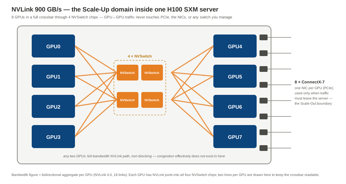
The bandwidth picture, with one correction to the source’s comparison table:
| Interconnect | Bandwidth (per GPU/NIC) | Convention | Scope |
|---|---|---|---|
| NVLink 4.0 (H100 SXM) | 900 GB/s | aggregate, both directions | intra-node GPU↔GPU |
| NVLink 5.0 (GB200) | 1,800 GB/s | aggregate, both directions | intra-node / intra-rack |
| NDR 400G InfiniBand | ~50 GB/s (~100 GB/s bidir) | per direction (per NIC) | cross-node |
| 400GbE Ethernet | ~50 GB/s (~100 GB/s bidir) | per direction (per NIC) | cross-node |
| PCIe Gen5 x16 | ~64 GB/s (~128 GB/s bidir) | per direction | same host, cross-NUMA |
Fact-check note: the source table compared NVLink’s bidirectional aggregate (900 GB/s = 18 links × 25 GB/s × 2 directions) against a NIC’s unidirectional rate (400 Gb/s = 50 GB/s), which overstates the ratio. Normalized consistently, the honest gap at the H100 generation is roughly 9× (450 vs ~50 GB/s per direction; 900 vs ~100 GB/s aggregate) — and about double that for Blackwell against the same 400G NIC. The conclusion survives the correction: this is not a gap engineering can close, because you cannot pull NVLink between racks; the physical form factor is the boundary.
Latency tells the same story: NVLink end-to-end sits in the sub-microsecond range (a microbenchmark-literature figure — NVIDIA publishes no official NVLink latency spec), while well-tuned cross-node RDMA lands between 1 and 5 µs. For synchronous collectives, latency is additive — every rank waits, and the microseconds compound with scale.
The operational consequence: when NCCL detects that all GPUs of a communicator share one NVLink domain, it routes the whole collective over NVLink — automatically, no configuration. Overriding it is possible but pointless: forcing that traffic onto the NIC is a performance regression, not a fix. Inside the 8-GPU domain there is nothing for a network engineer to configure or troubleshoot — an AllReduce there generates zero frames on any wire you own. That is also the trap in single-node benchmarking: if the numbers look wrong, the RoCEv2 config is not the suspect, because the traffic never used it.
9.2 The ninth GPU: where Scale-Out begins
The ninth GPU does not fit in the chassis, and from that point part of every collective takes this path:
GPU HBM → PCIe → RDMA NIC (CX7) → optics → leaf/spine switch → optics → RDMA NIC → PCIe → GPU HBM
Three structural changes arrive at once:
- Latency jumps an order of magnitude. Sub-µs NVLink becomes 1–5 µs RDMA on every cross-node hop of every synchronous collective.
- Per-GPU bandwidth falls ~9× (450 → ~50 GB/s per direction, using consistent units). The cliff is unavoidable; topology decides how much of the remainder is usable. Rail-optimized design uplinks each of the server’s 8 NICs to a different leaf switch, so 8 GPUs running one AllReduce get 8 independent parallel uplink paths that sum — instead of contending for a single uplink. It is the fabric-side mirror of NCCL’s own GPU→nearest-NIC assignment from section 8.5.
- Congestion starts existing. NVSwitch made it a non-issue; an Ethernet fabric carrying AllReduce incast is the opposite — many-to-one bursts pile up queues, and without PFC/ECN discipline the result is drops, RDMA go-back-N retransmits, and training throughput falling off a cliff. Everything from my RoCEv2 posts — PFC/ECN thresholds and headroom, the end-to-end DSCP contract — is the daily work of this domain.
Inside 8 GPUs the network engineer has no seat at the table; beyond 8, every configuration decision lands directly in training throughput.
9.3 Hybrid parallelism: mapping the primitives onto the two domains
Real large-model training runs several parallelisms at once, and each has a different traffic personality. This is where sections 4–5 (what each primitive moves, and which parallelism calls it) meet this section (what each domain costs):
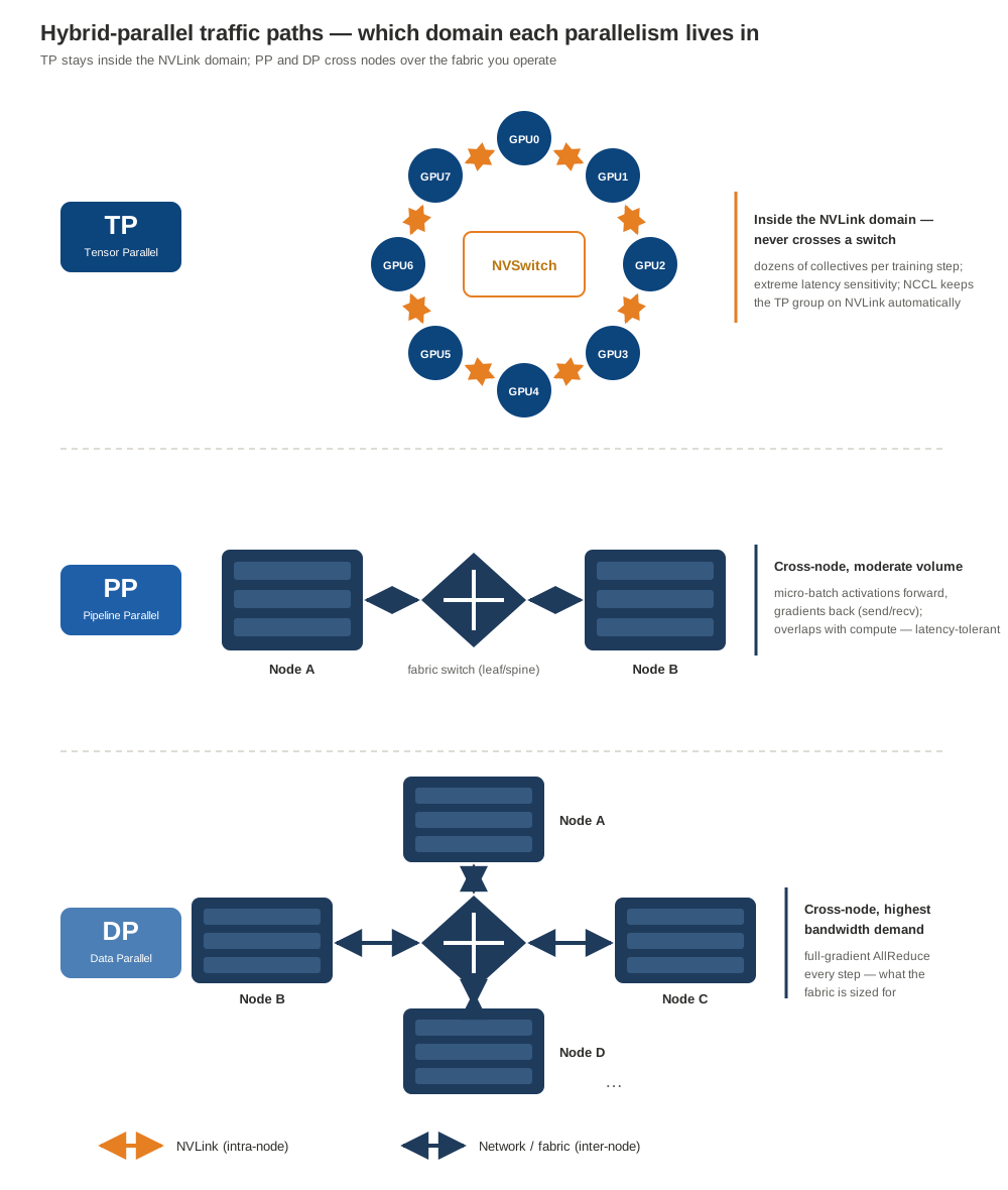
- TP (tensor parallel) slices the matrix math inside each Transformer layer and communicates dozens of times per training step — AllReduce/AllGather/ReduceScatter at extreme frequency, acutely latency-sensitive. NCCL keeps TP groups on NVLink automatically, and “TP degree ≤ NVLink domain size” is a hard placement rule: a TP group that straddles servers pays network latency an order of magnitude above NVLink on its hottest path. The misconfiguration signature is worth memorizing: when topology detection or process binding is wrong and TP silently spills onto the network, training runs far below reference, nothing reports an error, and NIC traffic sits much higher than the traffic model predicts. The wrongness is visible only to someone who knows what should never be on the wire at all.
- PP (pipeline parallel) hands micro-batch activations between adjacent stages — send/recv, cross-node, moderate volume, deliberately overlapped with compute, so it tolerates fabric latency far better than TP.
- DP (data parallel) is the bandwidth story and what Scale-Out fabrics are sized for: every step, every replica AllReduces the full gradient set. A 70B model in mixed precision carries ~140 GB of gradients; at DP=32, each GPU moves
2 × 31/32 × 140 GB ≈ 271 GBthrough its links per step — the Ring AllReduce arithmetic from 6.2 at production scale. Multiplied by steps per day, that is the number the capacity plan must survive. - MoE adds AlltoAll — four per MoE layer per step — many small, unevenly sized, latency- and balance-sensitive messages: the hardest pattern for an ECMP fabric to carry well.
The general placement rule, in one sentence: put the high-frequency communicator groups inside the fast domain first — TP within one NVLink/NVSwitch domain, DP across nodes, MoE’s expert parallelism across nodes only if the AlltoAll fabric can carry it, and pipeline-stage boundaries never on the worst-bandwidth path. This “topology mapping of the parallelism strategy” routinely buys more end-to-end performance than any NCCL environment variable.
9.4 The network engineer’s core work, by cluster size
- Single node, 8 GPUs — the baseline. The network is not the bottleneck; the job is baselining:
nvidia-smi topo -mshowingNV#everywhere,all_reduce_perf(nccl-tests) compared against NCCL’s reference numbers, results recorded as the baseline every later scale step is judged against. - 8–64 GPUs (2–8 servers). The network becomes the critical path — the scale where most engineers first feel the fabric in training throughput. Rail-optimized topology; RoCEv2 parameters aligned end to end (PFC on the RDMA priority, ECN thresholds, DSCP marking identical on NIC and switch — misalignment shows up as visible jitter in large-batch AllReduce); and an
ib_write_bw/ib_send_bwend-to-end bandwidth validation against link theory before any business benchmark runs. - 64–512 GPUs (8–64 servers). Real traffic engineering: two-tier spine-leaf or fat-tree with oversubscription no worse than ~2:1 (training forgives far less than inference); ECMP hashing validated under AllReduce-shaped load; on InfiniBand, evaluate Adaptive Routing — congestion-aware path selection whose published gains over static routing on congested fat-trees range from ~10% to ~28% depending on workload and topology (NVIDIA’s whitepaper measures bisection efficiency rising from 80% to 96%).
- 512+ GPUs. Every flaw not exposed earlier now amplifies. Adaptive Routing becomes mandatory rather than optional. On InfiniBand, SHARP is worth serious evaluation at this scale — it offloads AllReduce aggregation into the switches themselves (SHARPv2 streaming aggregation since Quantum HDR, SHARPv3 on Quantum-2; requires the SHARP Aggregation Manager, typically run under UFM; the fabric-side realization of section 6.4’s CollNet path), with measurable gains in latency and bandwidth consumption at thousand-GPU scale. On RoCEv2, PFC storm protection is a first-class design item: a fabric-wide PFC storm can stall everything, so configure PFC Watchdog to detect abnormal persistent PFC and automatically break losslessness before the avalanche.
9.5 The Scale-Up boundary is moving
The 8-GPU boundary is a property of the H100 generation, not a law. GB200 NVL72 connects 72 GPUs — 36 Grace-Blackwell superchips, each pairing one Grace CPU with two Blackwell GPUs — into a single rack-scale NVLink 5.0 domain: the rack behaves like one giant accelerator, and the network engineer’s entry point moves from “beyond 8 GPUs” to “beyond 72”. NVLink Fusion pushes further, licensing NVLink attachment to non-NVIDIA silicon.
The durable design rule: the intervention point is not a fixed GPU count — it is wherever the deployed platform’s Scale-Up domain ends. Inside that boundary, NVSwitch and NCCL own the problem. Outside it, you do.
10. Anatomy of one NCCL operation
Internals evolve by version, but a typical communication passes four phases — and each phase has its own failure modes (section 15).
- Initialization. The runtime launches processes and assigns ranks → one rank generates the Unique ID, the control plane distributes it → all ranks create communicators → bootstrap establishes initial connections and exchanges peer information → NCCL probes GPUs, NVLink, PCIe, CPUs, NICs, plugins → builds the topology and searches ring/tree/channel structures → each rank establishes P2P, shared-memory, or network connections and allocates buffers. Initialization is a distributed cooperative process: one rank missing, a rank-number conflict, an unreachable port, or an early exit leaves everyone else waiting.
- Operation submission.
ncclAllReduce()picks the execution plan from the collective type, datatype and reduction op, message size, communicator topology, available algorithms/protocols/channels, and user configuration — then enqueues work on the CUDA stream. With the Group API, NCCL collects the batch and plans it as one unit. - GPU and proxy coordination. Intra-node NVLink/P2P paths are driven mainly by GPU kernels — but cross-node communication also needs NCCL’s CPU proxy threads to drive the NIC: posting sends and receives, polling completion queues, making plugin progress. “NCCL is a GPU library” does not mean the CPU is uninvolved: wrong core binding, CPU contention, or a tight container CPU quota degrades cross-node NCCL directly.
- Completion. Stream work after the collective proceeds only when the kernels and transfers finish. On a network error, peer exit, or timeout, the framework must query the asynchronous error and decide whether to abort the communicator and the job — NCCL does not guarantee the surviving ranks of a crashed group can carry on; the standard recovery is tearing the group down and rebuilding it (what elastic-training systems automate).
10.1 Multi-stream and asynchronous execution: making communication non-blocking
The four phases describe one operation. What decides real training speed is what the GPU does while phase 3 runs: wait, or keep computing?
The problem. A naive training step is serial — forward → AllReduce → backward → AllReduce → next layer — and in that synchronous shape the GPU idles through every AllReduce, waiting for the transfer. For many models communication is 30% or more of step time, which means a GPU spending nearly a third of its life waiting:
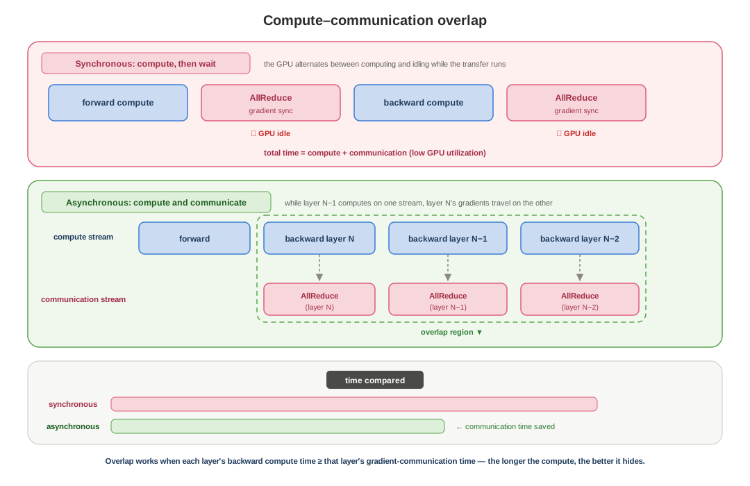
The dual-stream answer. NCCL rides CUDA’s stream mechanism (section 3.5): a compute stream runs the forward/backward kernels while a separate communication stream runs the collectives, and the two execute concurrently. While the communication stream grinds through layer N’s AllReduce, the compute stream is already producing layer N−1’s gradients. PyTorch DDP is exactly this loop — gradients materialize back-to-front, each finished bucket is enqueued on the communication stream immediately, and compute never stops (section 11.3 has the bucket mechanics and their size trade-off). Analogy: you keep cooking (compute) while the dishwasher runs (communication) — by the time the next course is prepped, the previous one’s dishes are clean.
In theory, when each layer’s AllReduce finishes before the compute stacked above it does, communication is fully hidden and training time ≈ pure compute time. The catch is the ratio: shallow layers and small batches produce AllReduces that outlive their compute, and the unhidden tail sticks out — which is precisely why topology (sections 8–9) and message coalescing (14.3) matter as much as they do.
Fewer kernel launches. Every communication operation launches a CUDA kernel, and a swarm of small operations pays that launch tax over and over. NCCL batches: the Group API (section 11.1) plans grouped operations together and submits them as fewer launches, and within one collective many chunks ride a single kernel — launch overhead stays amortized instead of dominating.
What asynchrony costs. Overlap is not free of rules. Buffer lifetime: the compute stream must not overwrite memory the communication stream is still reading. Synchronization points: results are usable only after the stream dependency is honored — work.wait(), a recorded event, or the blunt torch.cuda.synchronize() (section 3.5’s contract). Grouped submission: mutually dependent operations go between ncclGroupStart()/ncclGroupEnd() (section 4.4). Frameworks wrap all three so users rarely touch them — but these seams are exactly where misconception 5 and the section 15.2 hangs live.
11. Using it: CUDA and PyTorch
11.1 The CUDA C skeleton
The core multi-process AllReduce flow — the Unique ID distribution is a pseudo-function standing in for MPI, sockets, or a store:
#include <stdio.h>
#include <cuda_runtime.h>
#include <nccl.h>

#define CUDACHECK(cmd) do {                              \
  cudaError_t e = (cmd);                                 \
  if (e != cudaSuccess) {                                \
    printf("CUDA error %s:%d: %s\n",                     \
           __FILE__, __LINE__, cudaGetErrorString(e));   \
    exit(EXIT_FAILURE);                                  \
  }                                                      \
} while (0)

#define NCCLCHECK(cmd) do {                              \
  ncclResult_t r = (cmd);                                \
  if (r != ncclSuccess) {                                \
    printf("NCCL error %s:%d: %s\n",                     \
           __FILE__, __LINE__, ncclGetErrorString(r));   \
    exit(EXIT_FAILURE);                                  \
  }                                                      \
} while (0)

void run(int globalRank, int worldSize, int localRank,
         size_t count) {
  CUDACHECK(cudaSetDevice(localRank));

  ncclUniqueId id;
  if (globalRank == 0) {
    NCCLCHECK(ncclGetUniqueId(&id));
  }

  // distribute rank 0's id to every process via MPI, TCP, or a distributed store
  broadcastUniqueId(&id, sizeof(id), globalRank);

  ncclComm_t comm;
  NCCLCHECK(ncclCommInitRank(&comm, worldSize, id, globalRank));

  cudaStream_t stream;
  CUDACHECK(cudaStreamCreate(&stream));

  float *sendbuff = nullptr;
  float *recvbuff = nullptr;
  CUDACHECK(cudaMalloc(&sendbuff, count * sizeof(float)));
  CUDACHECK(cudaMalloc(&recvbuff, count * sizeof(float)));

  initializeInput(sendbuff, count, globalRank, stream);

  NCCLCHECK(ncclAllReduce(
      sendbuff,
      recvbuff,
      count,
      ncclFloat,
      ncclSum,
      comm,
      stream));

  // ncclAllReduce returning only means the operation is enqueued
  CUDACHECK(cudaStreamSynchronize(stream));

  CUDACHECK(cudaFree(sendbuff));
  CUDACHECK(cudaFree(recvbuff));
  CUDACHECK(cudaStreamDestroy(stream));
  NCCLCHECK(ncclCommDestroy(comm));
}
When one thread submits for multiple GPUs, group the calls — the Group API is not just call-overhead reduction; it lets NCCL treat the batch as one submission and schedule it in parallel instead of blocking call by call:
NCCLCHECK(ncclGroupStart());
for (int i = 0; i < ndev; ++i) {
  CUDACHECK(cudaSetDevice(devices[i]));
  NCCLCHECK(ncclAllReduce(
      sendbuff[i], recvbuff[i], count,
      ncclFloat, ncclSum, comms[i], streams[i]));
}
NCCLCHECK(ncclGroupEnd());
11.2 PyTorch
import os
import torch
import torch.distributed as dist

def main():
    local_rank = int(os.environ["LOCAL_RANK"])
    torch.cuda.set_device(local_rank)

    dist.init_process_group(backend="nccl")

    rank = dist.get_rank()
    tensor = torch.tensor([rank + 1.0], device="cuda")

    dist.all_reduce(tensor, op=dist.ReduceOp.SUM)
    torch.cuda.synchronize()

    print(f"rank={rank}, result={tensor.item()}")
    dist.destroy_process_group()

if __name__ == "__main__":
    main()
torchrun --standalone --nproc-per-node=4 demo.py
Four ranks start with 1, 2, 3, 4; after AllReduce-Sum every rank prints 10.
11.3 Why DDP overlap works — and what the bucket size trades
DDP holds a full replica per GPU. Gradients materialize back-to-front during backprop, so DDP groups parameters into buckets and launches an async AllReduce the moment a bucket’s gradients are ready:
backward computes bucket 3
        ↓ gradients ready
launch bucket 3 AllReduce ─────┐
        ↓                      │ communication
continue computing bucket 2    │ overlaps compute
        ↓                      │
launch bucket 2 AllReduce ─────┘
Too-small buckets → many small collectives, latency-dominated. Too-large buckets → the first AllReduce starts late and overlap shrinks. DDP tuning is therefore never just NCCL tuning: bucket size, gradient-readiness order, and the model’s computation graph are all part of it.
12. Measuring NCCL properly
12.1 Latency, algbw, busbw
Three metrics appear in every NCCL benchmark:
- Latency — completion time of one operation.
- Algorithm bandwidth (algbw) — user data volume ÷ time.
- Bus bandwidth (busbw) — algbw normalized by the collective’s theoretical link traffic, so it can be compared against hardware bus capability.
For a Ring AllReduce of M total bytes (M as in section 6.2), the per-rank traffic is 2(P−1)/P × M, so:
busbw = algbw × 2 × (P − 1) / P
The factor differs per collective — nccl-tests’ PERFORMANCE.md derives each one (it writes n for the rank count this post calls P):
| Collective | busbw factor on algbw | Why |
|---|---|---|
| AllReduce | 2(n−1)/n | every element moves twice through the ring (6.2) |
| ReduceScatter / AllGather | (n−1)/n | every element moves once, minus the local share |
| AlltoAll | (n−1)/n | each rank keeps 1/n of its own data local |
| Broadcast / Reduce | 1 | everything must leave (or reach) the root — the root is the bottleneck |
| SendRecv | 1 | a plain point-to-point copy |
The point of the normalization, in the doc’s own words: busbw exists so you can “compare it with the hardware peak bandwidth, independently of the number of ranks used”, and “the bus bandwidth should reflect the speed of the hardware bottleneck: NVLink, PCI, QPI, or network.” The companion rule: look at time for small sizes — that is the constant launch-and-latency overhead — and at bandwidth for large ones. Never compare raw algbw one-to-one against a unidirectional link spec.
12.2 nccl-tests: the official benchmark
nccl-tests is NVIDIA’s own suite, and its first sentence states the double mission: the tests “check both the performance and the correctness” of NCCL operations. The build produces eleven binaries — one per pattern:
all_reduce_perf   all_gather_perf    broadcast_perf   reduce_scatter_perf
reduce_perf       alltoall_perf      alltoallv_perf   scatter_perf
gather_perf       sendrecv_perf      hypercube_perf
(alltoallv_perf exercises the variable-count pattern via the grouped-send/recv composition from section 4.3 — NCCL itself still has no AlltoAllV collective.)
Building is one make; point it at non-default installs with CUDA_HOME/NCCL_HOME, and build with make MPI=1 MPI_HOME=/path/to/mpi for multi-node runs (MPI is how the tests span processes and nodes):
git clone https://github.com/NVIDIA/nccl-tests.git && cd nccl-tests
make MPI=1 MPI_HOME=/path/to/mpi CUDA_HOME=/path/to/cuda NCCL_HOME=/path/to/nccl
The rank math is the one rule everyone trips over: total ranks (= CUDA devices) = processes × threads per process (-t) × GPUs per thread (-g) — the process count comes from mpirun, not from the tool. The two canonical invocations from the README:
./build/all_reduce_perf -b 8 -e 128M -f 2 -g 8                 ! one process driving 8 GPUs (single node)
mpirun -np 64 -N 8 ./build/all_reduce_perf -b 8 -e 8G -f 2 -g 1  ! 8 nodes x 8 GPUs, one rank per GPU
The arguments that matter day to day (defaults in parentheses):
| Group | Flags |
|---|---|
| Size sweep | -b min / -e max (both default 32M — always set them), -f multiply per step or -i fixed increment |
| GPU mapping | -t threads per process (1), -g GPUs per thread (1) |
| Operation | -o sum/prod/min/max/avg/all (Sum), -d datatype (Float), -r root rank for rooted collectives (0) |
| Iterations | -n timed iters (20), -w warmup iters, not timed (1), -m operations aggregated per iteration (1) |
| Correctness | -c check iterations (1 — validation is on by default; slow at large scale, -c 0 to disable) |
| Modifiers | -G capture as CUDA Graph and replay, -R buffer registration (1 local, 2 symmetric), -z blocking mode, -T per-test timeout, -a report avg/min/max across ranks (MPI builds) |
One environment variable of the suite itself deserves a network engineer’s attention: NCCL_TESTS_SPLIT partitions the GPUs into groups running the same operation in parallel — e.g. NCCL_TESTS_SPLIT="MOD 8" on 8-GPU nodes runs eight parallel operations, each with one GPU per node, so the traffic is purely inter-node: a clean way to load the fabric without any NVLink component (bandwidth is then reported per group).
12.3 Reading the output
Each run prints three parts: a preamble, one row per message size, and a footer. The preamble — the nccl-tests version, the parameter line, and a # Using devices block with every rank’s host, PID, and PCI bus id — is worth a glance to confirm the rank↔GPU↔node mapping you intended. Each data row holds two column groups, out-of-place and in-place (section 5.2’s distinction), each with time, algbw, busbw, and #wrong. The footer:
#wrongandOut of bounds valuesare the correctness half: input buffers are generated by the suite’sverifiablelibrary, which “carefully craft[s] floating point input to produce exactly predictable output”, so every received element is compared against the exact expected value — a nonzero count fails the run.Avg bus bandwidthis the arithmetic mean of every busbw measurement in the run — a single regression-tracking number (andNCCL_TESTS_MIN_BWturns it into a pass/fail gate, useful in burn-in pipelines).
The header block, from a real capture (a two-node V100 run posted in nccl-tests issue #107):
# nThread 1 nGpus 1 minBytes 1310720000 maxBytes 1310720000 step: 1048576(bytes) warmup iters: 5 iters: 20 validation: 1
#
# Using devices
#   Rank  0 Pid   1320 on ip-172-31-20-228 device  0 [0x00] Tesla V100-SXM2-16GB
#   Rank  0 Pid   2066 on ip-172-31-22-230 device  0 [0x00] Tesla V100-SXM2-16GB
#
#                                                       out-of-place                       in-place
#       size         count      type   redop     time   algbw   busbw  error     time   algbw   busbw  error
#        (B)    (elements)                       (us)  (GB/s)  (GB/s)            (us)  (GB/s)  (GB/s)
And this particular capture is a broken run, diagnosable from the header alone — which is exactly why the issue was filed as “How to understand the result?”: both processes report Rank 0, meaning the binary was not built with MPI=1, so each node ran its own independent single-GPU “collective” (the NCCL maintainer’s reply in the thread says precisely that: “running two independent single GPU tests”). In the original paste the whole preamble even appears twice — each un-synchronized process printed its own — one more symptom of the same problem, elided above for readability. The data rows confirm it — busbw prints 0.00 because the AllReduce factor 2(n−1)/n is zero at n=1, and the in-place half reports a nonsensical ~2,000,000 GB/s “algbw” — two petabytes per second — for what is a no-op. First lesson of reading nccl-tests output: check # Using devices before believing any number.
A healthy run at scale, published in NVIDIA’s HPC-X user manual — 1,024 GPUs across 128 nodes, IB SHARP/CollNet enabled (section 6.4 live):
mpirun -np 1024 -map-by ppr:8:node -x NCCL_COLLNET_ENABLE=1 -x NCCL_ALGO=CollNet \
    ./nccl-tests/build/all_reduce_perf -b 4 -e 2G -f 2 -g 1 -w 50 -n 50

           4             1   float     sum    44.53    0.00    0.00  3e-05    44.21    0.00    0.00  3e-05
           8             2   float     sum    45.42    0.00    0.00  3e-05    45.85    0.00    0.00  3e-05
          16             4   float     sum    46.34    0.00    0.00  3e-05    45.84    0.00    0.00  2e-05
          32             8   float     sum    46.20    0.00    0.00  2e-05    46.56    0.00    0.00  2e-05
          64            16   float     sum    46.00    0.00    0.00  2e-05    48.33    0.00    0.00  2e-05
         128            32   float     sum    48.77    0.00    0.01  2e-05    47.23    0.00    0.01  2e-05
         256            64   float     sum    47.88    0.01    0.01  2e-05    47.85    0.01    0.01  2e-05
         512           128   float     sum    51.44    0.01    0.02  3e-05    48.66    0.01    0.02  3e-05
        1024           256   float     sum    51.27    0.02    0.04  4e-05    51.78    0.02    0.04  4e-05
        2048           512   float     sum    57.93    0.04    0.07  4e-05    56.45    0.04    0.07  4e-05
        4096          1024   float     sum    57.32    0.07    0.14  4e-05    93.51    0.04    0.09  4e-05
        8192          2048   float     sum    106.4    0.08    0.15  4e-05    59.70    0.14    0.27  4e-05
       16384          4096   float     sum    103.0    0.16    0.32  4e-05    58.23    0.28    0.56  4e-05
       32768          8192   float     sum    74.85    0.44    0.87  4e-05    137.8    0.24    0.48  4e-05
       65536         16384   float     sum    96.71    0.68    1.35  4e-05    92.89    0.71    1.41  4e-05
      131072         32768   float     sum    115.6    1.13    2.27  4e-05    120.7    1.09    2.17  4e-05
      262144         65536   float     sum    197.7    1.33    2.65  4e-05    167.6    1.56    3.13  4e-05
      524288        131072   float     sum    222.7    2.35    4.70  4e-05    239.2    2.19    4.38  4e-05
     1048576        262144   float     sum    280.9    3.73    7.46  4e-05    197.7    5.30   10.60  4e-05
     2097152        524288   float     sum    218.0    9.62   19.22  4e-05    213.9    9.81   19.59  4e-05
     4194304       1048576   float     sum    257.6   16.28   32.53  4e-05    254.7   16.47   32.90  4e-05
     8388608       2097152   float     sum    354.3   23.68   47.31  4e-05    523.5   16.02   32.02  4e-05
    16777216       4194304   float     sum    505.9   33.16   66.26  4e-05    484.1   34.66   69.24  4e-05
    33554432       8388608   float     sum    639.2   52.50  104.89  4e-05    678.6   49.45   98.80  4e-05
    67108864      16777216   float     sum   1358.2   49.41   98.72  4e-05   1048.6   64.00  127.87  4e-05
   134217728      33554432   float     sum   1737.2   77.26  154.37  4e-05   1777.6   75.51  150.86  4e-05
   268435456      67108864   float     sum   4359.5   61.58  123.03  4e-05   4262.3   62.98  125.83  4e-05
   536870912     134217728   float     sum   5619.7   95.53  190.88  4e-05   5699.0   94.20  188.22  4e-05
  1073741824     268435456   float     sum    12169   88.23  176.30  4e-05    11508   93.30  186.42  4e-05
  2147483648     536870912   float     sum    22618   94.94  189.70  4e-05    21814   98.44  196.70  4e-05
# Out of bounds values : 0 OK
# Avg bus bandwidth    : 41.2497
This one table carries every lesson of the section. The latency floor: a 4-byte AllReduce across 1,024 GPUs completes in ~45 µs, and the whole left half of the sweep is pinned there regardless of size — pure launch-and-synchronization overhead. The S-curve: busbw climbs from the floor through the megabyte range and plateaus around 190–197 GB/s at gigabyte sizes — as NVIDIA’s tuning guidance puts it, a healthy system “level[s] off at the line rate of the hardware”, and the plateau is what you compare against the bottleneck link (12.1); a plateau far below it, or a curve that never flattens, is where the sections 13–15 toolbox comes in. The error column (older releases print the max relative error for floating-point checks; current ones print the #wrong element count) stays at ~4e-05 — float rounding, not corruption — and the footer’s Out of bounds values: 0 OK is the pass. And Avg bus bandwidth: 41.25 shows why that footer number is a regression tracker rather than a headline: it averages the entire sweep, latency floor included, so it sits far below the 190 GB/s the fabric actually delivers.
For calibration on the single-node ladder, NVIDIA’s own published numbers for what topology buys: ~5 GB/s across CPU sockets over shared memory, ~12 GB/s with PCIe P2P, and NVLink aggregating far beyond (132 GB/s already on Volta’s six links) — the measured version of section 8’s transport ladder.
12.4 Methodology
A trustworthy measurement controls at least: GPU model and clock state; NCCL/CUDA/driver/network-driver versions; node count, GPUs per node, rank mapping; GPU-CPU-NIC NUMA affinity; the message-size range; warm-up; whether compute overlaps; whether algorithm/protocol are auto-selected; IB/RoCE port speeds, link state, congestion; and whether anything else shares the PCIe, NVLink, or network. And never record a single peak number: training traffic spans many bucket sizes, so the deliverable is the full message-size → latency/bandwidth curve.
Two more lenses for interpreting what that curve measures, both second nature to a network engineer:
- What the number is an indicator of migrates with scale. On 1–4 nodes, nccl-tests mostly measures the servers — NVLink, PCIe, NUMA binding, NCCL’s own efficiency. Around 8–32 nodes it becomes a hybrid of node and fabric. Beyond ~64 nodes the fabric dominates, and the busbw curve is effectively a network-capability indicator: rail balance, congestion control, and ECMP behavior show up in it before anything GPU-side does. The same 41 GB/s average means completely different things at each of those scales.
- Judge stability by the tail, not the mean. A synchronized collective completes when its slowest rank does (section 15.6), so a fabric that averages well but jitters badly trains slowly. nccl-tests has per-iteration statistics for exactly this —
-I 1reportsi_min/i_max/i_p99/i_cv%per size — and across repeated runs the P95/P99 spread matters more than the average. A scaling sweep should degrade smoothly as nodes are added; a sharp drop at one node count is an inflection worth chasing (an oversubscription tier, a hash imbalance, a rail asymmetry — section 15.4’s ladder).
13. The environment-variable toolbox
NCCL exposes many environment variables for device selection, logging, algorithm control, and diagnostics. Semantics move between versions — verify against the docs of the version you run.
13.1 Logging and diagnostics
| Variable | Effect |
|---|---|
NCCL_DEBUG | Log level: VERSION, WARN, INFO, TRACE |
NCCL_DEBUG_SUBSYS | Select subsystems: INIT, GRAPH, NET, COLL, P2P, SHM, ENV, TUNING, … |
NCCL_DEBUG_FILE | Write per-process logs to files (supports hostname/PID placeholders like %h, %p) |
The standard diagnostic combination:
export NCCL_DEBUG=INFO
export NCCL_DEBUG_SUBSYS=INIT,GRAPH,NET
This answers, from the logs alone: which NIC NCCL actually chose; whether a network plugin loaded; whether GPUDirect RDMA is active; how many channels were built; which intra-node and inter-node connections are in use.
13.2 Network and device selection
| Variable | Effect |
|---|---|
NCCL_SOCKET_IFNAME | Specify or exclude socket network interfaces |
NCCL_IB_HCA | Specify or exclude IB/RoCE HCAs and ports |
NCCL_IB_DISABLE | Disable the IB/RoCE transport (falls back to socket) — for isolation testing |
NCCL_NET | Select the network implementation or plugin; valid values depend on the environment |
NCCL_NET_GDR_LEVEL | Topology-distance threshold up to which GPUDirect RDMA is used |
NCCL_CROSS_NIC | Whether rings/trees may cross NIC rails; exact semantics per version docs |
NCCL_SOCKET_IFNAME and NCCL_IB_HCA use their own matching rules — prefix match, ^ exclusion, = exact — not general regular-expression syntax.
13.3 Intra-node path control
| Variable | Effect |
|---|---|
NCCL_P2P_DISABLE | Disable GPU P2P — to test whether the P2P path is the problem |
NCCL_P2P_LEVEL | Topology distance up to which P2P is allowed |
NCCL_SHM_DISABLE | Disable the shared-memory transport |
These are made for bisection-style fault isolation: if disabling P2P fixes the program, suspect GPU P2P, IOMMU, virtualization, or driver topology. But a diagnostic fallback is not a fix — disabling features costs performance and should never survive into production configuration.
13.4 Algorithm, protocol, channels
| Variable | Effect |
|---|---|
NCCL_ALGO | Restrict/exclude algorithms: Ring, Tree, CollNetChain, CollNetDirect, NVLS, NVLSTree, PAT (versions vary; settable per collective since 2.24) |
NCCL_PROTO | Restrict/exclude protocols (Simple, LL, LL128) |
NCCL_NVLS_ENABLE | NVLink SHARP: 0 off; 2 (default) enable when the device reports multicast support; 1 enable without that check — neither fails on unsupported hardware, both fail if NVLS resources cannot be allocated |
NCCL_COLLNET_ENABLE | Enable the CollNet plugin path (default 0) |
NCCL_MIN_NCHANNELS | Floor on the channel count |
NCCL_MAX_NCHANNELS | Ceiling on the channel count |
The tuning discipline: (1) baseline on automatic selection; (2) confirm from logs what was actually selected; (3) change one variable at a time; (4) test the full message-size range, not one size; (5) validate on the real model — a microbenchmark optimum does not guarantee end-to-end throughput.
13.5 NCCL_* vs TORCH_NCCL_*
PyTorch has its own family of TORCH_NCCL_* variables — watchdog, async error handling, timeout diagnostics, the Flight Recorder. They configure ProcessGroupNCCL, not the NCCL library:
NCCL_*        → NVIDIA NCCL library behavior
TORCH_NCCL_*  → PyTorch ProcessGroupNCCL behavior
Keeping the two namespaces straight avoids a whole category of “I set the variable and nothing changed” confusion.
13.6 The quick-reference card
The handful you actually reach for, on one card:
| Variable | What it does | When to reach for it |
|---|---|---|
NCCL_DEBUG=INFO | Print topology, transport, and channel decisions | The first move in any investigation (13.1, 15.1) |
NCCL_ALGO=Ring / =Tree | Pin the algorithm | A/B tests and fault isolation only — the cost model already picks Ring for large messages and Tree for small (6.6) |
NCCL_PROTO=Simple | Pin the protocol | When an LL/LL128 bug is suspected — the docs discourage setting it otherwise (sections 7, 13.4) |
NCCL_MIN_NCHANNELS | Raise the channel floor | Multi-NIC nodes where too few channels underfeed the rails (8.7); NCCL_MIN_NRINGS is its pre-2.5 name |
NCCL_NTHREADS | CUDA threads per channel’s block | Practically never — the default tracks the GPU generation |
NCCL_P2P_LEVEL | Distance cap for GPU P2P | Debugging when NVLink/P2P looks unused (13.3, 15.7) |
Note: cards like this circulate with “set Ring for large messages, Tree for small” as standing tuning advice. In NCCL that is what the cost model already does per message size — pinning is a diagnostic, not a configuration strategy (sections 6.6 and 13.4).
14. Optimization beyond environment variables
14.1 Bind rank, GPU, CPU, and NIC correctly
The most fundamental and most-skipped item is the device mapping:
local rank      → the correct GPU
process CPU     → the NUMA node next to that GPU
network traffic → the NIC/HCA next to that GPU
Checklist: did each process cudaSetDevice correctly; is local rank still right after CUDA_VISIBLE_DEVICES renumbering; does the container expose the expected GPU, RDMA, and shared-memory devices; is CPU pinning squeezing all ranks onto a few cores; are GPU and HCA on the same CPU socket.
14.2 Hide communication rather than accelerate it
For most training workloads the goal is not NCCL at theoretical peak — it is communication time hidden behind compute: right-sized DDP gradient buckets, launched as early as readiness allows; FSDP prefetching the next layer’s parameters; communication on its own CUDA stream with event-managed dependencies; no cudaDeviceSynchronize() on the hot path; sensible micro-batch scheduling in pipeline parallel.
14.3 Coalesce small messages
Small messages pay launch latency, kernel launch, synchronization, and network round trips; a swarm of tiny collectives runs at a fraction of link bandwidth. Levers: tensor fusion, gradient buckets, the Group API, coarser parallel partitioning, and CUDA Graphs (after confirming the capture support of your NCCL and framework versions). Coalescing has its own cost — waiting for more tensors reduces overlap — so the target is balance, not “as big as possible”.
14.4 Map the parallelism to the topology
Section 9.3’s placement rule, restated as the optimization it is: high-frequency groups inside the NVLink domain, DP across nodes, MoE across nodes only with an AlltoAll-capable fabric, stage boundaries off the worst links. This regularly outperforms any environment-variable tuning.
14.5 Check the network, not just NCCL
Cross-node anomalies frequently originate outside NCCL: an HCA port below target rate; RoCE PFC/ECN misconfiguration; IB routing or congestion; inconsistent MTU; wrong GID index or interface selection; mismatched GPUDirect RDMA kernel modules (DMA-BUF / peer memory); VMs, containers, or security policy blocking RDMA devices; multi-tenant sharing of the same uplink. The NCCL log tells you which path it used — it does not replace network-layer monitoring and switch diagnostics.
15. Troubleshooting
15.1 Stuck in initialization
Typical causes: a rank never started or exited early; duplicate/missing ranks or inconsistent world_size; inconsistent Unique ID; hostname resolution or bootstrap network unreachable; firewalls, security groups, or Kubernetes NetworkPolicy; nodes picking mutually unreachable Docker/virtual/management interfaces; inconsistent software stacks or device visibility across nodes. First move:
export NCCL_DEBUG=INFO
export NCCL_DEBUG_SUBSYS=INIT,NET
(If a subsystem name is not recognized by your version, drop back to NCCL_DEBUG=INFO alone.)
15.2 Hangs at a collective
The most common cause is not a slow network — it is ranks disagreeing about the operation sequence:
Rank 0: AllReduce(A) → AllGather(B)
Rank 1: AllGather(B) → AllReduce(A)
Ranks in one communicator must enter operations in a compatible order. Then check the rest of section 3.7’s contract: element counts, datatypes, root rank consistency; a rank that skipped the collective on an exception; a conditional branch that only some ranks executed; multiple threads submitting to one communicator in nondeterministic order.
15.3 unhandled system error and friends
The message is a symptom, not a cause. Behind it may be: an inaccessible NIC/HCA; RDMA registration failure; a broken GPUDirect path; insufficient shared memory; a peer process that died; ABI mismatch across driver/CUDA/NCCL/plugin; or a container missing device, IPC, memlock, or permission configuration. Judge from the earliest NCCL WARN in the logs, kernel logs, RDMA device state, and the framework logs together — never from the last error line alone.
15.4 Fast on one node, slow across nodes
Work the ladder in order:
- Establish single-node and dual-node baselines separately with nccl-tests.
- Confirm from logs whether cross-node traffic went over IB/RoCE or fell back to socket —
NET/Socketwhere you expected RDMA means fix the RDMA path first, not the ring count. - Confirm the intended HCA ports were selected.
- Verify GPUDirect RDMA is in effect.
- Check GPU–NIC NUMA distance and process core binding.
- Check port speeds, error counters, drops, congestion.
- Scale out gradually and note the scale where performance first falls off.
The classic scale-out culprits from the RoCEv2 world, with their signatures:
- PFC absent or half-configured. PFC on the switch but the NIC trusts PCP while the fabric marks DSCP — PFC never triggers, congestion drops packets, go-back-N retransmits stall the collective:
mlnx_qos -i eth0                   ! current QoS/trust configuration
ethtool -S eth0 | grep pause       ! PFC pause counters
- ECN thresholds unreasonable. Too low: normal traffic constantly throttled. Too high: queues are deep before marking starts and PFC ends up doing ECN’s job. Starting point: mark at ~20–30% of port buffer and tune against measurement — buffer sizes differ enough between switch generations that absolute values do not transfer.
- ECMP hash imbalance. Fabric-wide utilization moderate, but a few links pinned at 100% with drops or PFC storms exactly there. Under AllReduce-shaped load, spine per-port utilization should be near-uniform; deviation beyond ~30% means the hash configuration needs work.
15.5 /dev/shm too small
Container defaults can be tiny, and both NCCL’s intra-node path and the DataLoader’s worker processes use shared memory:
df -h /dev/shm
Docker, Kubernetes, and container runtimes each size shared memory differently. Do not reach for NCCL_SHM_DISABLE before confirming the actual error path — it may mask the problem at a performance cost.
15.6 Intermittent jitter
A collective finishes when its slowest rank does — “NCCL got slower” often means “some rank arrived later”. Candidate causes: GPU downclocking or thermal/power limits; the CPU proxy thread preempted; congestion or a noisy neighbor; one rank computing slower; MoE token imbalance; NUMA auto-balancing, IRQ, or background-task interference; uneven traffic across rails; data loading intermittently starving some ranks.
15.7 Scale-Up domain checks
Three intra-node problems, none visible from the network side:
- NCCL detected the wrong topology. Symptom: training >20% below reference on identical hardware, network clean, NIC traffic higher than expected (section 9.3’s TP-spill signature). Check:
nvidia-smi topo -m ! GPU pairs should show NV# (# = NVLink link count); SYS = no NVLink path, NCCL fell back to PCIe/network
- PCIe/NUMA affinity wrong. Two NUMA nodes, 4 GPUs + NICs each; a process bound to the wrong node pays cross-NUMA tax on every host transfer:
numactl --hardware        ! NUMA topology
lstopo                    ! visualize PCIe/NUMA relationships
- NVLink under its rated bandwidth. Rare — usually an NCCL/driver mismatch or BIOS NVLink settings. Watch real NVLink counters via
dcgm-exporteragainst the theoretical peak.
16. Six misconceptions
- “NCCL installed ⇒ RDMA used.” RDMA depends on hardware, drivers, container device exposure, plugins, and runtime configuration; when unavailable, NCCL silently falls back to socket. Only the logs tell you the real path.
- “NVLink bandwidth = AllReduce bandwidth.” Nominal, unidirectional, bidirectional, per-GPU aggregate, algorithm, and bus bandwidth are six different numbers, and collectives add reduction, synchronization, chunking, and topology constraints. Never use a marketing spec as the expected benchmark value.
- “Forcing Ring / adding channels is always faster.” Small messages often want Tree and low-latency protocols; extra channels cost overhead. Baseline on auto-selection and verify any forced setting with benchmarks.
- “A stuck collective is an NCCL bug.” Inconsistent operation order between ranks, an exited process, mismatched tensor sizes, and divergent control flow are all more common (section 15.2).
- “The call returned, so communication finished.” NCCL operations are asynchronous stream submissions (section 3.5); read results only after the stream dependency is satisfied.
- “Fast microbenchmark ⇒ fast training.” End-to-end speed also hangs on overlap, message-size distribution, rank load balance, redundant synchronization in the framework, data loading and the CPU, and the topology mapping of the parallelism strategy.
17. Training traffic vs inference traffic
In large-model systems NCCL is not just “the gradient library” — it is the shared data plane of every parallelism strategy:
Data Parallel        →  gradient synchronization
Tensor Parallel      →  intra-layer activation / partial-result exchange
Pipeline Parallel    →  activation and gradient transfer between stages
FSDP / ZeRO          →  sharded parameter, gradient, and optimizer-state communication
Expert Parallel      →  token redistribution across experts
Training jobs stack several of these at once, so each process holds multiple communicators — and scheduling must keep the groups from serializing against each other or entering overlapping groups in different orders (a communicator-level deadlock in the making).
Inference uses the same primitives — TP’s per-layer AllReduce/AllGather, PP’s send/recv, MoE’s AlltoAll, multi-GPU sampling and logits aggregation — but cares about different numbers: single-token latency and tail latency. Decode-phase messages are small and extremely frequent, so a configuration tuned for training’s large-message bandwidth is not automatically right for inference. And KV-cache migration across instances is not necessarily NCCL’s job at all: when the peers are not fixed ranks, nodes join and leave dynamically, or data moves between GPU, CPU, SSD, and object storage, systems reach for NIXL, UCX, raw RDMA, object-storage interfaces, or an in-house transport layer. NCCL’s home ground is high-performance GPU collectives within a fixed communication group.
18. Summary and first-response toolkit
Five layers, and you understand NCCL:
- Communication semantics — what AllReduce, AllGather, ReduceScatter, Broadcast, AlltoAll, and Send/Recv each solve (sections 4–5).
- Communication organization — how rank, communicator, collective, channel, and CUDA stream structure an operation (section 3).
- Algorithms and protocols — Ring/Tree/CollNet/NVLS decide the structure; Simple/LL/LL128 decide the transmission (sections 6–7).
- Topology and transport — how paths are chosen among NVLink, PCIe, shared memory, RDMA, socket (sections 8–9).
- System-level performance — the end-to-end number also depends on parallelism strategy, message granularity, overlap, NUMA binding, and the network fabric (sections 12–15).
The working method, in order — not “set twenty environment variables and hope”:
confirm topology and device mapping
        ↓
establish layered baselines with nccl-tests
        ↓
confirm the real communication path from NCCL logs
        ↓
locate the bottleneck: compute, synchronization, intra-node link, or network
        ↓
change one variable at a time, verify end to end
When training is “slow” and the network is a suspect, in this order:
NCCL_DEBUG=INFO <job>              ! which collective, what sizes, which transport was chosen - answers are usually in here
nvidia-smi topo -m                 ! NV# everywhere it should be
all_reduce_perf -b 8 -e 8G -f 2 -g 8   ! nccl-tests vs the recorded single-node baseline (without -g it runs 1 rank - a no-op, see 12.3)
ib_write_bw / ib_send_bw           ! end-to-end RDMA bandwidth vs link theory, before blaming the model
dcgm-exporter                      ! NVLink + NIC counters over time, not point samples
And the four one-liners this post compresses into: AllReduce = ReduceScatter + AllGather (explains Ring AllReduce and FSDP at once); DDP uses AllReduce, FSDP uses AllGather+ReduceScatter, MoE uses AlltoAll, pipeline uses send/recv; memory has three layers (user buffers have formulas, NCCL buffers need differential measurement, framework counters exclude NCCL); and a hang means checking that every rank entered the same collective with the same count and datatype before touching any tuning knob.
References
- NVIDIA NCCL User Guide — Collective Operations, In-place Operations, Environment Variables
- NVIDIA — NCCL GitHub repository, nccl-tests
- PyTorch — Distributed documentation
- NVIDIA — GB200 NVL72
- CloudSwitch — How to read NCCL test results (the scale-migration and tail-latency lenses in 12.4)
- Related posts on this blog: RoCE QoS concepts and packet examples, End-to-end RoCEv2: Nexus, Cumulus, ConnectX, RDMA performance tuning