
TP, PP, DP: How Large Models Actually Use Multiple GPUs
Note: this post started from several explainers found via web search, was cross-checked against the Megatron-LM paper and the vLLM documentation, and adds the memory math, communication costs, and decision rules those explainers leave out. It is the deployment-side companion to the NCCL and NVLink notes, which cover what actually moves on the wire underneath these strategies.
When you deploy a large model, you keep seeing configurations like “Qwen-72B, 8 GPUs” or “Qwen-32B, 2× L20” — and the natural question is: how is one model split across several cards, and how do the cards cooperate? Multi-GPU is not “the VRAM adds up.” The GPUs have to be organized, and there are three basic ways to organize them — Tensor Parallelism (TP), Pipeline Parallelism (PP), and Data Parallelism (DP) — each solving a different problem.
Contents — 8 sections
1. Why one GPU is not enough
Multi-GPU deployment exists to solve exactly two problems, and everything else in this post follows from which of the two you have:
Problem 1: the model is too big  → one GPU cannot HOLD it     → TP / PP
Problem 2: the users are too many → one GPU cannot SERVE them  → DP
Problem 1 — the model doesn’t fit
The dominant cost is the weights. In FP16/BF16 every parameter takes 2 bytes:
70B model:   70 × 10⁹ params × 2 B  ≈ 140 GB   (weights alone)
32B model:   32 × 10⁹ params × 2 B  ≈  64 GB
7B model:     7 × 10⁹ params × 2 B  ≈  14 GB
An NVIDIA L20 has 48 GB; an A100/H100 has 80 GB. A 70B model in FP16 does not fit on any single card — not even close. And weights are only the start; serving also needs KV cache, which grows with every concurrent request and every token of context:
KV cache per token = 2 (K and V) × layers × kv_heads × head_dim × bytes

Llama-3-70B (GQA):  2 × 80 × 8 × 128 × 2 B ≈ 320 KB per token
  → one 8K-token request  ≈ 2.6 GB
  → one 128K-token request ≈ 40 GB   (half a GPU for a single conversation)
So the practical planning number is weights + KV cache + activations + ~10–20% overhead. When that total exceeds one card, the model must be split — that is model parallelism, and TP and PP are its two flavors.
Problem 2 — the model fits, but the traffic doesn’t
A 7B model runs comfortably on one GPU. But when a few hundred users arrive at once, requests queue and latency explodes. Memory is not the bottleneck — compute and KV-cache capacity per instance are. The fix is not to split the model but to copy it: run several complete instances and spread the requests. That is data parallelism.
2. TP — Tensor Parallelism: one model, every GPU computes every layer
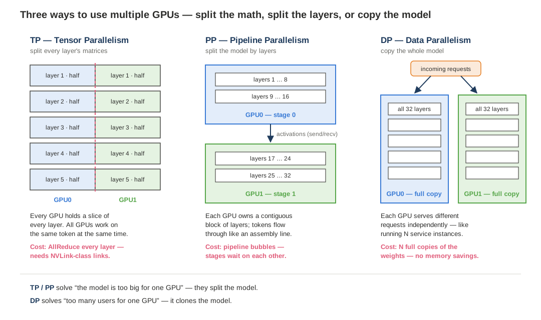
TP attacks Problem 1 by splitting inside each layer. A transformer is mostly large matrix multiplications (input × weight matrix), and a matrix multiplication can be computed in pieces: cut the weight matrix in half, let each GPU multiply against its half, then combine the results. With TP=2, every weight matrix in every layer is half on GPU0 and half on GPU1; both GPUs work on the same token at the same time.
The classic construction is Megatron-LM’s column/row split. For the MLP block Y = GeLU(X·A)·B:
- A is split by columns. Each GPU computes
GeLU(X·Aᵢ)— a complete, valid slice of the intermediate activation. No communication needed. - B is split by rows. Each GPU multiplies its activation slice by its rows of B, producing a partial sum of the final output.
- One AllReduce adds the partial sums, and both GPUs have the full result.
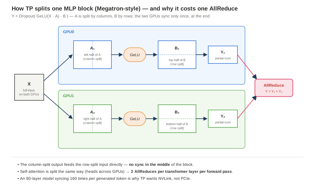
The column-then-row ordering is the whole trick: the output of the column-split layer feeds the row-split layer directly, so an entire two-matmul block costs a single sync. Self-attention splits the same way — attention heads are distributed across GPUs (column-parallel QKV projection, row-parallel output projection) — so a transformer layer costs 2 AllReduces per forward pass: one for attention, one for the MLP.
That is also TP’s price tag. An 80-layer model generating one token performs ~160 AllReduces, every token, and each one blocks compute until it completes:
- Latency-critical, very frequent communication. This is why TP lives inside an NVLink domain (≈900 GB/s per H100) and degrades badly over plain PCIe (Gen4 x16, ≈64 GB/s bidirectional — what an L20 box has) — the NCCL post, section on traffic profiles has the per-workload numbers.
- The practical rule: TP does not cross the node boundary.
tensor_parallel_size≤ GPUs per node, essentially always. - TP prefers power-of-two degrees (2, 4, 8) because attention heads and hidden dimensions must divide evenly across the group.
What TP buys: memory per GPU drops by the TP factor (140 GB ÷ 4 ≈ 35 GB — an A100 can hold it), and because all GPUs multiply in parallel, each individual forward pass gets faster. TP is the only one of the three that reduces per-token latency, which is why it is the default for latency-sensitive serving. The configurations from the intro decode to exactly this: Qwen-32B (64 GB weights) on 2× 48 GB L20 is TP=2; Qwen-72B on 8 GPUs is typically TP=8 or TP=4 combined with something else.
3. PP — Pipeline Parallelism: one model, split by layers
Where TP splits the math of every layer, PP splits the model by layers. A 32-layer model with PP=2:
GPU0:  embedding + layers 1–16     (stage 0)
GPU1:  layers 17–32 + output head  (stage 1)

user input → GPU0 computes its 16 layers → hands activations to GPU1
           → GPU1 computes its 16 layers → token out
Like a factory line: workshop A does the first half of the work, passes the part to workshop B. The communication profile is completely different from TP: a stage passes one activation tensor per micro-batch to the next stage — a point-to-point send/recv, moderate volume, and only at stage boundaries instead of every layer. PP therefore tolerates slow interconnects gracefully: it is the natural strategy across nodes and on PCIe-only boxes.
The weakness is the bubble. While GPU0 processes the first batch, GPU1 sits idle; when the last batch drains, GPU0 idles. Splitting each batch into m micro-batches keeps more stages busy simultaneously, but the fill/drain cost never disappears:
bubble fraction = (p − 1) / (m + p − 1)      p = stages, m = micro-batches

p=4, m=4  →  3/7  ≈ 43% idle
p=4, m=16 →  3/19 ≈ 16% idle
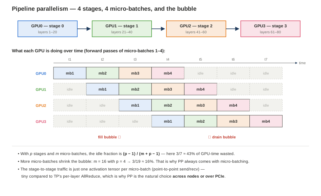
In serving, continuous batching plays the role micro-batches play in training — with enough concurrent requests in flight, every stage always has work, and the bubble mostly disappears at high load. At low load (a single interactive request), PP adds pipeline latency without making any single token faster, which is why PP is a throughput tool, not a latency tool.
Compared head-to-head with TP: PP needs cheap interconnect and scales to arbitrary depth (any number of layers ÷ any number of stages, even uneven splits), but per-request latency doesn’t improve and utilization depends on keeping the pipe full. TP makes every token faster but demands NVLink and even divisibility. Hence the standard combination in the next sections: TP inside the node, PP across nodes.
4. DP — Data Parallelism: one model, copied N times
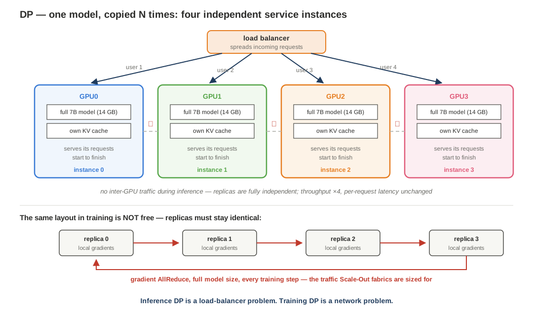
DP is not model splitting at all. It solves Problem 2 — the model fits, the traffic doesn’t — by running complete, independent copies:
GPU0: full 7B model     user 1 → GPU0
GPU1: full 7B model     user 2 → GPU1
GPU2: full 7B model     user 3 → GPU2
GPU3: full 7B model     user 4 → GPU3
It is exactly “run 4 service instances behind a load balancer.” During inference the replicas exchange no model traffic whatsoever — each has its own weights and its own KV cache. Throughput scales almost linearly with replica count; latency of an individual request does not change at all. The cost is memory: N replicas store the weights N times.
Two practical notes that the simple picture hides:
- Serving frameworks make DP a first-class dimension. vLLM offers
--data-parallel-sizewith an internal load balancer, a hybrid per-node mode, and a fully external mode where each rank is its own endpoint behind your own router. For dense models, plain external replicas (Kubernetes + N vLLM pods) are often operationally simplest; internal DP matters most for MoE models, where attention runs data-parallel while expert layers form one bigDP × TPgroup (see §6). - DP in training is a different animal. There the replicas must stay mathematically identical, so every step ends with an AllReduce over the full gradient set — at DP=32 on a 70B model that is ~271 GB through each GPU’s links per step, the number Scale-Out fabrics are sized for (worked through in the NCCL post). ZeRO/FSDP push further by sharding optimizer state, gradients, and parameters across the DP group. None of that traffic exists in inference DP — replicas never talk.
5. Real deployments combine them
Production rarely uses one strategy alone, because a real deployment usually has both problems at once: the model is too big and the traffic is high. The classic 8-GPU recipe for a 70B model:
TP=4 × DP=2 on 8 GPUs

GPU0–3:  replica 0 — one model instance, each GPU holds 1/4 of every layer
GPU4–7:  replica 1 — a second identical instance
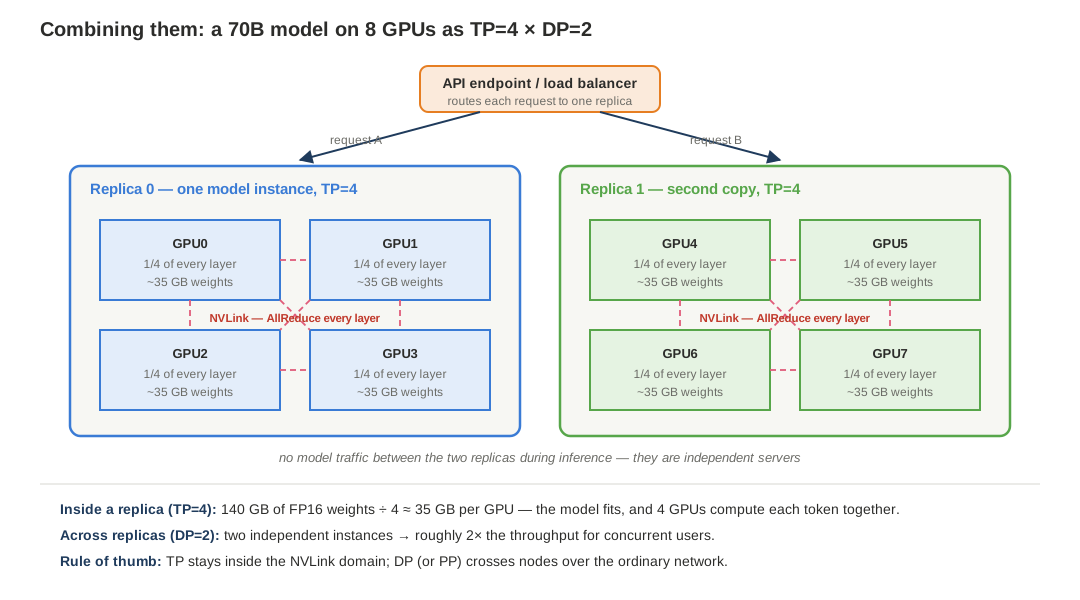
TP=4 solves “too big” (140 GB ÷ 4 ≈ 35 GB per GPU, fits an 80 GB card with room for KV cache); DP=2 solves “too many users” (double the throughput). Whether TP=8 or TP=4 × DP=2 wins on the same 8 GPUs is a latency/throughput trade: TP=8 gives the fastest single token and the largest pooled KV space, TP=4 × DP=2 usually gives more aggregate throughput because each token’s AllReduces run in a smaller, cheaper group.
When one node is not enough, PP joins in — TP inside each node where NVLink is, PP across nodes where only Ethernet/InfiniBand is:
# one node, 4 GPUs — model fits in the node: plain TP
vllm serve Qwen/Qwen2.5-72B-Instruct --tensor-parallel-size 4

# 2 nodes × 8 GPUs — model too big for one node: TP intra-node × PP inter-node
vllm serve <model> --tensor-parallel-size 8 --pipeline-parallel-size 2 \
    --distributed-executor-backend ray

# model fits one GPU, traffic is high: DP replicas behind one endpoint
vllm serve <model> --data-parallel-size 4
Training stacks the same dimensions one deeper: Megatron-style 3D parallelism is DP × PP × TP — TP=8 inside each node, PP chaining nodes into one model instance, DP replicating that whole arrangement dozens of times, with ZeRO sharding layered on the DP dimension. The organizing principle is identical to inference: the most communication-hungry dimension (TP) gets the fastest links, the most tolerant one (DP) gets the slowest.
6. Beyond the big three: EP and SP
Two more letters show up in modern configs, both answers to newer model shapes:
- EP (Expert Parallelism) — for MoE models (DeepSeek-V3/R1, Mixtral, Qwen3-MoE). Experts are distributed across GPUs, and each token is routed to its top-k experts via All-to-All exchanges. Since only a fraction of experts activate per token, the sparse expert weights shard naturally by expert rather than by matrix slice. The common large-scale MoE serving pattern is DP attention + EP/TP experts (vLLM:
--enable-expert-parallel), with the caveat that all ranks in the expert group must step forward together, so idle DP ranks execute dummy passes. - SP (Sequence/Context Parallelism) — splits along the sequence dimension. In training it shards the activations TP leaves replicated (LayerNorm/dropout regions); as context parallelism it spreads a very long sequence (128K+) across GPUs so no single card holds the whole KV cache of one request — the fix for that 40 GB single-request number from §1.
Neither replaces TP/PP/DP; they compose with them. A DeepSeek-scale serving config can read DP=32 attention, EP=32 experts across four nodes — still the same two problems, sliced along model-specific axes.
7. How to choose
The decision is mostly mechanical once you know three numbers: model memory (weights + expected KV cache), memory per GPU, and GPUs per node.
| Situation | Choice | Why |
|---|---|---|
| Model fits one GPU, low traffic | Single GPU | Parallelism only adds overhead |
| Model fits one GPU, high traffic | DP replicas | Linear throughput scaling, zero sync cost |
| Model too big for one GPU, fits one node | TP = GPUs per node | NVLink absorbs the per-layer AllReduces; lowest latency |
| Model too big for one node | TP (intra-node) × PP (inter-node) | Each dimension matched to its interconnect |
| PCIe-only server, or uneven GPU count | PP over TP | Stage handoffs tolerate slow links; uneven layer splits are fine |
| Too big and high traffic | TP × DP (e.g. TP=4 × DP=2) | Split first until it fits, then clone for throughput |
| MoE model at scale | EP (+ DP attention) | Shard by expert, not by matrix |
| 100K+ contexts dominate | add SP/CP | One request’s KV cache no longer fits one card |
| Large-scale training | DP(ZeRO/FSDP) × PP × TP | 3D parallelism; DP carries the gradient traffic |
And the two-line summary the whole topic compresses to:
Model too big   → split it   → TP (split the math) / PP (split the layers)
Users too many  → copy it    → DP
Deployment sizing is never “VRAM is short, add GPUs” — it is model size + concurrency + interconnect capability jointly deciding how the GPUs are organized.
8. Quick reference
Memory estimate for serving:
total ≈ weights + KV cache + activations + overhead

weights (GB)          ≈ params(B) × 2         (FP16/BF16; ×1 for FP8, ×0.5 for INT4)
KV per token (bytes)  = 2 × layers × kv_heads × head_dim × dtype_bytes
per-GPU weights       = weights ÷ (TP × PP)
Communication profile of each dimension (what the fabric must survive):
| Dimension | Primitive | Frequency | Interconnect need |
|---|---|---|---|
| TP | AllReduce / AllGather | Every layer, every token | NVLink/NVSwitch — intra-node only |
| PP | send/recv (P2P) | Once per stage per micro-batch | Modest — fine across nodes |
| DP (inference) | none | — | none (just a load balancer) |
| DP (training) | AllReduce over gradients | Once per step, full model size | The Scale-Out fabric’s sizing case |
| EP | All-to-All | Every MoE layer | High — the hot spot of MoE serving |
References
- Megatron-LM: Training Multi-Billion Parameter Language Models Using Model Parallelism — the column/row-parallel construction in §2
- vLLM — Parallelism and Scaling and Data Parallel Deployment — flags and multi-node guidance
- PyTorch — Large Scale Transformer training with Tensor Parallel
- Sebastian Raschka — KV cache calculations — the per-token formula in §1
- NVIDIA — Mastering LLM Techniques: Inference Optimization
- Companion post: NCCL and NVLink Notes — the communication layer all of this runs on